Chapter 2 Data understanding and preparation
2.1 Dataset
To create a model that will predict whether a client application represents a risk or not, we worked on a data set from our client containing data on 1000 past credit applications, described by the following variables:
CHK_ACCT: The checking account status of the applicant in Deutsche Mark (DM).
DURATION: The duration of the credit in months.
HISTORY: The credit history of the applicant.
NEW_CAR: Purpose of the credit.
USED_CAR: Purpose of the credit.
FURNITURE: Purpose of the credit.
RADIO/TV: Purpose of the credit.
EDUCATION: Purpose of the credit.
RETRAINING: Purpose of the credit.
AMOUNT: The credit amount.
SAV_ACCT: The average balance in savings account in Deutsche Mark (DM).
EMPLOYMENT: If the applicant is employed and since how long.
INSTALL_RATE: The installment rate as percentage of disposable income.
MALE_DIV: If the applicant is male and divorced.
MALE_SINGLE: If the applicant is male and single.
MALE_MAR_or_WID: If the applicant is male, married or widowed.
CO_APPLICANT: If the applicant has a co-applicant.
GUARANTOR: If the applicant has a guarantor.
PRESENT_RESIDENT: If the applicant is a resident and since how many years.
REAL_ESTATE: If the applicant owns real estate.
PROP-UNKN-NONE: If the applicant owns no property (or unknown).
AGE: Age of the applicant.
OTHER_INSTALL: If the applicant has other installment plan credit.
RENT: If the applicant rents.
OWN_RES: If the applicant owns residence.
NUM_CREDITS: Number of existing credits of the applicant at our client bank.
JOB: The nature of the applicant’s job.
NUM_DEPENDENT: Number of people for whom liable to provide maintenance.
TELEPHONE: If the applicant has a phone in his or her name.
FOREIGN: If the applicant is a foreign worker.
RESPONSE: If the credit application is rated as “Good” or “Bad”.
2.2 Exploratory Data Analysis
In this part, we thoroughly explored the data set to get a better understanding. The goal of the exploratory data analysis was to observe and interpret our data thanks to visualization methods, like plots.
2.2.1 Inacurracies
By doing an exploratory data analysis, we found some inaccuracies and in agreement with our client, we changed them as follow:
- One observation of the variable “AGE”: 75 instead of 125 years old.
- One observation of the variable “EDUCATION”: 1 instead of -1.
- One observation of the variable “GUARANTOR”: 1 instead of 2.
2.2.2 Unbalanced observations
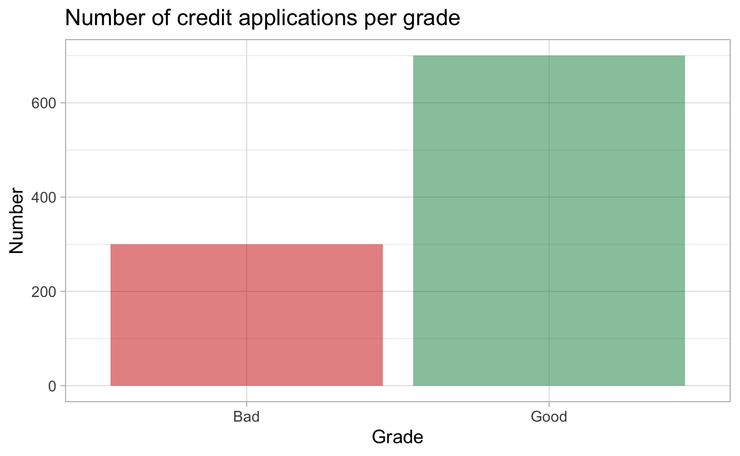
To start, we noticed an important point to consider: the data set is heavily unbalanced. As you can see on the following plot, it contains 700 credit applications rated as good versus 300 credit applications rated as bad. We will need to balance the data set for our modelling.
Taking the last point into account, we also decided to split the database in 2 parts: the first part considered only the good clients, and the second part considered only the bad clients. This will help us to study the particularities of each profile.
2.2.3 Visualization
We chose to show some specifics variables as they are the ones we will be using in the modelling part.
To have a better visualization of our variables. We used some box plots or histograms showing the distribution of the data.
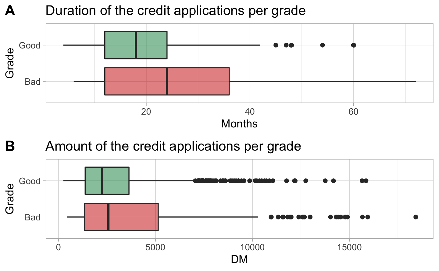
This first box plot A shows that bad clients mostly asked for longer duration credit than good clients. This could be a reason why they received a refusal. The second box plot B shows that most of the good clients asked for a smaller amount.
Then, we explored the distribution of the financial variables:
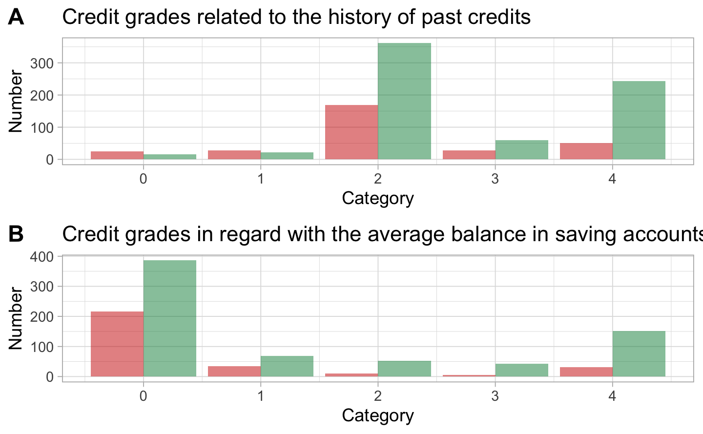
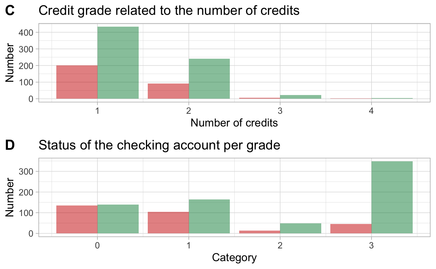
The first graph A represents the situation with past credits. The behavior for good and bad clients is almost the same which does not allow us to make a clear difference. On the graph B we can see that most of the clients have small savings or even no savings at all. Most of the clients have already 1 or 2 credits at this bank. Almost none of them ask for a third or fourth credit. On the histogram D we see that the amount of money on the account is not so important. Indeed, most of the good client do not even have a checking account.
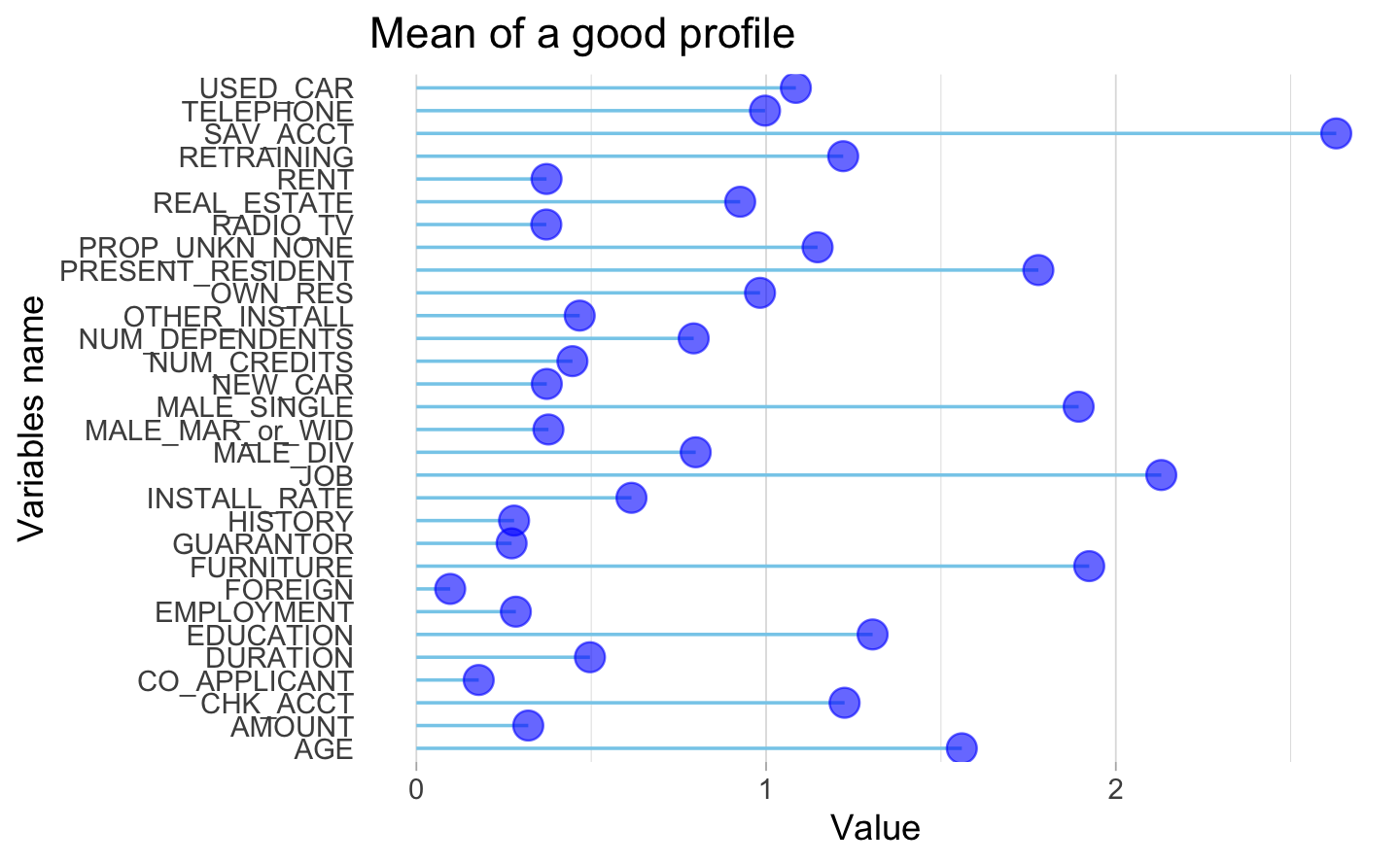
2.2.4 Profile of a good client
The following part of the project is focus on defining a typical profile of a good client. The goal is to define an average good client based on the average of all the variables defined.
First, we cleaned the data set created at the beginning which contain only good clients to have the average of each variable. Then, we created a plot with these average data.
The lollipop plot below represents the mean profile to be qualified as a good client. From these results, most of them asked for a new car, rented their flat but had real estate. The good client in average had a quite good amount of money and had a guarantor. These results are quite different than what we presented before.
2.2.5 Profile of a bad client
Then, we used exactly the same approach to build the typical profile of a bad client and identify the average variables that qualify a bad client in this bank.
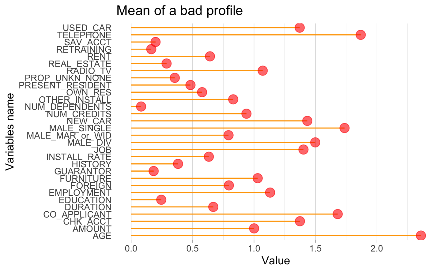
As we can see on the orange lollipop plot, the result is different. Most of the bad clients rented their flat. This criteria sounds really important to qualify a client. Almost all of them do not have any other credit in the bank and they have other installment plan credits. For further analysis, it will be more relevant to use the median instead of the mean to have more robust results.