Chapter 1 Consumer Behavior
1.1 The Axioms of Rational Choice
In order to make models for how consumers behave, we need to assume that they will act in a rational manner. In simple terms, this means that the consumers act in a consistent and predictable way. If consumer behavior were completely random and unpredictable, it would be impossible for us to model how they operate.
1.1.1 Preference Relations
Before we cover the main assumptions for rational behavior, we should take a look at the symbols we use to summarize a consumer’s preference for different goods.
Let’s say Karan has a choice between apples and oranges. If Karan always picks apples over oranges, we can say that he strictly prefers apples to oranges. Using symbols we rewrite this as \(Apples \succ Oranges\).
If a consumer strictly prefers good a over good b, we write: \[a \succ b\]
If Karan likes apples and oranges equally, we can say he is indifferent to the goods. We can then rewrite this as \(Apples \sim Oranges\).
If a consumer is indifferent between the two, we write: \[a \sim b\]
Lastly, if Karan likes his apples at least as much as he likes oranges, we can say that he weakly prefers apples to oranges. Using symbols we rewrite this as \(Apples \succsim Oranges\).
If a consumer weakly prefers good a over good b, we write: \[a \succsim b\] Why don’t we just use normal inequality symbols?
We use special preference symbols instead of regular inequalities because preferences aren’t really quantifiable. We can say for sure that \(2 \gt 1\), but we can’t say \(Apples \gt Oranges\) because it’s not absolute. Karan might like Apples more than Oranges, but Sarah might feel the opposite way.
1.1.2 Completeness
Our consumer, Karan, should be able to rank his preference for apples versus oranges; he can say he is indifferent or that he prefers one over the other.
For a set of goods, a and b, a consumer can rank their preferences, for example: \[a \succ b \quad or \quad a \sim b\]
1.1.3 Transitivity
If Karan likes apples more than oranges and likes oranges more than bananas, then Karan must like apples more than bananas.
If a consumer prefers a more then b and b more than c, then they must prefer a over c. \[if \quad a \succ b \quad and \quad b \succ c \implies a \succ c\]
1.1.4 Continuity
If Karan likes Pink Lady apples more than oranges, he should also like Honeycrisp apples more than oranges because the two apples are so similar.
If a consumer prefers a to b, they should also prefer goods almost identical to a to b. \[if \quad a \succ b \quad and \quad a \sim a^{\prime} \implies a^{\prime} \succ b\]
1.2 Utility Functions
To build quantitative models for consumer behavior, we need to have a method of assigning numerical values to different situations. The utility function gives us a way to organize consumers’ preferences by attaching numerical values to them.
A utility function is typically of the form \(U(input)= output\). The input is some consumable such as a bundle of goods, and the output is a numerical value assigned to that input, measured in utils.
1.2.1 The Arguments of a Utility Function
The inputs of a utility function can vary significantly because there are so many different situations or goods that we can compare and rank.
The most common input is \(q\), the quantity of a good or multiple goods. The function here measures levels of utility given by the different combinations of goods that an individual consumes. \[U(q_1, q_2, ... \thinspace ,q_n)\]
Another input is the combination of consumption, \(C\), and leisure, \(H\), where you can measure the levels of utility provided by different combinations of consumption and leisure; the amount consumed is directly related to the amount of time spent working (not spent leisurely) because greater hours worked implies more money available to consume goods and services. \[U(C,H)\]
A more interesting utility function exists when an individual is altruistic, meaning they care for the wellbeing of another. This utility function would consider the consumption of the individual and the consumption of whoever they care about. \[U(C_{individual}, C_{others})\]
1.2.2 Visualizing a Utility Function
In order to build some intuition about what exactly a utility function does, we should look at graphs to explore their structure.
Let’s take a utility function with the inputs being 2 different goods, \(x\) and \(y\), of the following form: \[U(x,y)=x \times y\]
1.2.2.1 Surface Plot
Figure 1.1: A surface plot of the utility function. Drag around on the graph to get a better look at the shape.
The surface plot provides a great way of exploring exactly how our function looks, but it can be impractical if not impossible to show on a piece of paper. As an alternative, we can use contour plots.
1.2.2.2 Contour Plot
Figure 1.2: A filled contour plot of the utility function.
A filled contour plot can be thought of as a surface plot that has been flattened to fit on a 2D plane. The color of the regions represents the value of utility changing based on the \(x\) and \(y\) values. The distinct lines each correspond to one constant value of the utility, \(\bar{U}\).
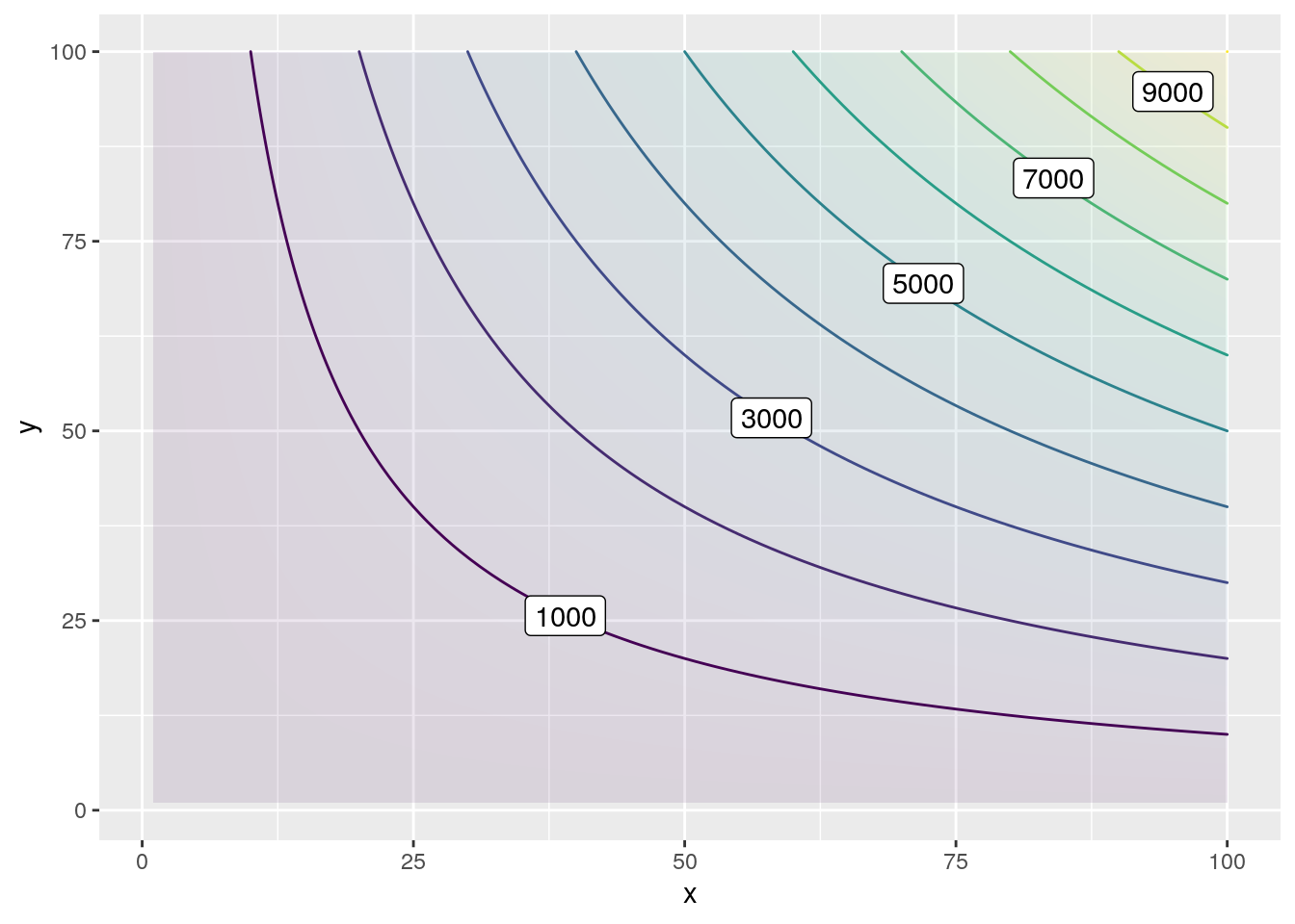
Figure 1.3: A line contour plot of the utility function
Taking the fill away leaves us with a plot that gives us a rough outline of what the utility function really looks like. These lines represent a constant value of utility, showing us the different bundles of good \(x\) and \(y\) that an individual can consume at a given \(\bar{U}\).
1.3 Indifference Curves
Let’s say \(U = q_{Apples}^{0.5} \times q_{Oranges}^{0.5}\) represents Karan’s utility function for apples and oranges. How much utility does Karan get from having 5 apples and 180 oranges? How about 20 apples and 45 oranges? The opposite? Plugging each of these bundles into our utility function, we see that they all give Karan the same utility of 30. Take a look at the graph below to find other bundles that give Karan a utility of 30:
Figure 1.5: Karan’s Bundles when \(U=30\)
This is what we call an indifference curve. Every point on the curve represents a bundle that gives us a particular utility, \(\bar{U}\); in this case \(\bar{U} = 30\). No matter what combination of apples and oranges Karan consumes from this graph, his utility will stay 30.
1.3.1 The Indifference Map
Why should we limit Karan’s utility to 30? What if his utility was 70? What if it were 10? The same way Karan has different bundles to keep \(\bar{U} = 30\), he has different bundles to keep his \(\bar{U}\) at different levels.
Figure 1.6: Karan’s Indifference Map
We call this graph an indifference map. It represents every possible bundle an individual can consume to keep their utility at a particular level. This graph should appear familiar to Figure 1.3, the line contour plot from Visualizing a Utility Function, because they are actually one and the same. Figure 1.3 is an simply an indifference map for the utility function \(U(x,y)=x \times y\) .
Making things clearer visually, we can see that points on indifference curves each have the same height when projected to the surface of the utility function.
Figure 1.7: Karan’s Indifference Curves Projected to the Utility Surface
1.4 Marginal Utility
Now we’ll take a look at marginal utility. You might remember from introductory micro that marginal utility describes the additional utility you get from consuming another unit of a good. In more mathematical terms we mean \(\frac{\Delta Total\thinspace Utility}{\Delta Quantity \thinspace Consumed}\), which we can rewrite using calculus as \(\frac{\mathrm{d} TU}{\mathrm{d} Q}\)
But you probably realized that the marginal utility you learned in introductory micro only accounts for one good. What are we supposed to do with utility equations that have several goods? We have to use partial differentiation. Partial differentiation is simply taking a derivative with respect to one variable while holding the others