Chapter 4 Chi-squared Distribution and Tests
4.1 chisq.test
- performs chi-squared contingency table tests and goodness-of-fit tests.
chisq.test(x, y = NULL, correct = TRUE,
           p = rep(1/length(x), length(x)), rescale.p = FALSE,
           simulate.p.value = FALSE, B = 2000)
x, y = NULL: the input can be two numeric vectors as x and y (can both be factors), or a matrix as x.correct: a logical indicating whether to apply continuity correction.
4.1.1 output components
- Dataset
# Example in A01
birthwt <- data.frame("Low" = c(21054, 27126), "Normal" = c(14442, 3804294), row.names = c("Dead at Year 1", "Alive at Year 1"))
birthwt
## Low Normal
## Dead at Year 1 21054 14442
## Alive at Year 1 27126 3804294chi <- chisq.test(birthwt)
chi##
## Pearson's Chi-squared test with Yates' continuity correction
##
## data: birthwt
## X-squared = 981695, df = 1, p-value < 2.2e-16# use dollar sign($) to specify output
chi$statistic # the value the chi-squared test statistic## X-squared
## 981695.2chi$parameter # the degrees of freedom## df
## 1chi$p.value## [1] 0chi$method## [1] "Pearson's Chi-squared test with Yates' continuity correction"chi$data.name## [1] "birthwt"chi$observed## Low Normal
## Dead at Year 1 21054 14442
## Alive at Year 1 27126 3804294chi$expected # the expected counts under the null hypothesis## Low Normal
## Dead at Year 1 442.2639 35053.74
## Alive at Year 1 47737.7361 3783682.26chi$residuals # the Pearson residuals, (observed - expected) / sqrt(expected).## Low Normal
## Dead at Year 1 980.10778 -110.08988
## Alive at Year 1 -94.33735 10.59637chi$stdres # standardized residuals, (observed - expected) / sqrt(V)## Low Normal
## Dead at Year 1 990.8294 -990.8294
## Alive at Year 1 -990.8294 990.82944.2 pchisq
- Density, distribution function, quantile function and random generation for the chi-squared (\(\chi^2\)) distribution with
dfdegrees of freedom and optional non-centrality parameterncp.
pchisq(q, df, ncp = 0, lower.tail = TRUE, log.p = FALSE)q: (vector of) quantile(s).df: degrees of freedom (non-negative, but can be non-integer).lower.tail: logical; if TRUE (default), probabilities are \(P[X \le x]\), otherwise, \(P[X > x]\).
4.2.1 Example
To find the p-value that corresponds with a \(\chi^2\) test statistic of 7 from a test with one degree of freedom:
pchisq(7, df=1, lower.tail = FALSE)## [1] 0.008150972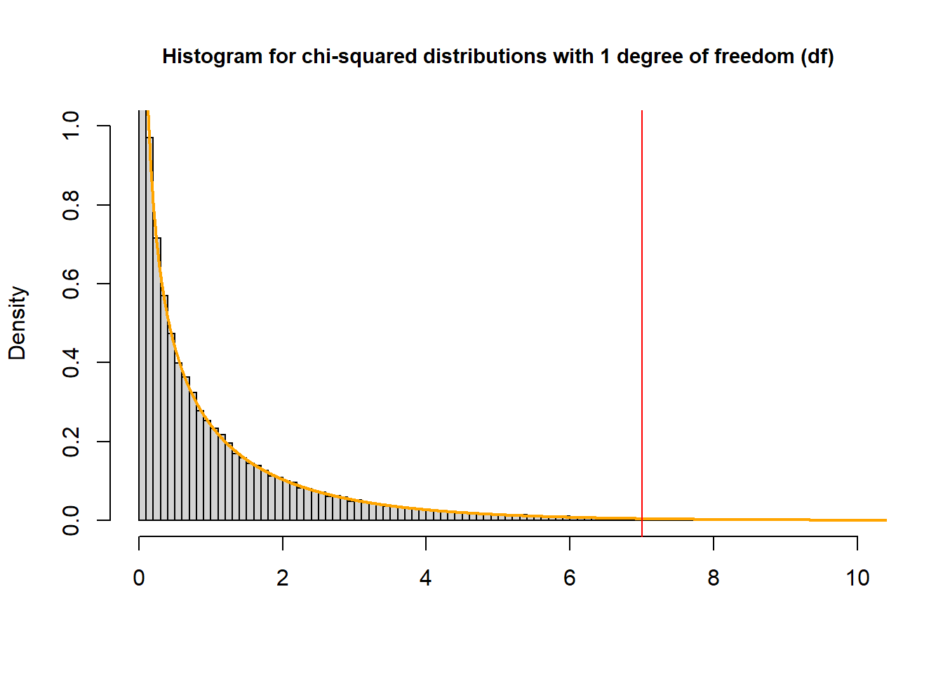
The P-value is the probability of observing a sample statistic as extreme as the test statistic – the area to the left of the red line – “upper” tail
We always set
lower.tail = FALSEwhen calculating P-value of \(\chi^2\) test.Another method to get the p-value
# default: lower.tail = TURE
1 - pchisq(7, df=1)
## [1] 0.0081509724.3 mantelhaen.test
Performs a Cochran-Mantel-Haenszel chi-squared test of the null that two nominal variables are conditionally independent in each stratum, assuming that there is no three-way interaction.
- To test the null hypothesis that the exposure is independent of the disease when adjusting for confounding, we can use
mantelhaen.test(x, y = NULL, z = NULL,
                alternative = c("two.sided", "less", "greater"),
                correct = TRUE, exact = FALSE, conf.level = 0.95)
Input data:
- A 3-dimensional contingency table in array form as
x - Or three factor objects with at least 2 levels as
x,y, andz.
- A 3-dimensional contingency table in array form as
correct = TRUE: Whether to apply continuity correction when computing the test statistic.exact = FALSE: Whether the Mantel-Haenszel test or the exact conditional test (given the strata margins) should be computed.
# example
dat <- foreign::read.dta("./_data/diet.dta")
tab <- with(dat, table(diet, mort, by = act))
# see general code for more information about the table
mantelhaen.test(tab)
##
## Mantel-Haenszel chi-squared test with continuity correction
##
## data: tab
## Mantel-Haenszel X-squared = 1.1249, df = 1, p-value = 0.2889
## alternative hypothesis: true common odds ratio is not equal to 1
## 95 percent confidence interval:
## 0.5228808 1.1789039
## sample estimates:
## common odds ratio
## 0.7851281