第 4 章 社会资本与精准扶贫
社会资本与精准扶贫
library(tidyverse)
library(here)
library(fs)
library(haven)
library(broom)
4.1 数据导入
我们选取了北京大学开放数据平台中的中国家庭追踪调查CFPS4的2014年数据。
cfps2014famecon <- read_dta("../data/2014AllData/Cfps2014famecon_170630.dta",
  encoding = "GB2312"
)

cfps2014adult <- read_dta("../data/2014AllData/cfps2014adult_170630.dta",
  encoding = "GB2312"
)
4.2 选取变量
筛选家庭数据库中相关的变量
- use: Cfps2014famecon_170630.dta
- keep: fid14, fa3, fa4, fa5, fa8, fa9, fs6_s_1-fs6_s_15
筛选成人数据库中相关的变量
- use: cfps2014adult_170630.dta
- keep: pid, fid14, cfps2012_latest_edu, qp201, qn12012, qn12013, qn12014, qn1011-qn1017
## 获取标签

library(purrr)
get_var_label <- function(dta) {
  labels <- map(dta, function(x) attr(x, "label"))
  data_frame(
    name = names(labels),
    label = as.character(labels)
  )
}
df_famecon <- cfps2014famecon %>%
dplyr::select(
fid14, fa3, fa4, fa5, fa8,
fa9, fs6_s_1:fs6_s_15
)
df_famecon %>% get_var_label()## # A tibble: 21 x 2
## name label
## <chr> <chr>
## 1 fid14 2014年家户号
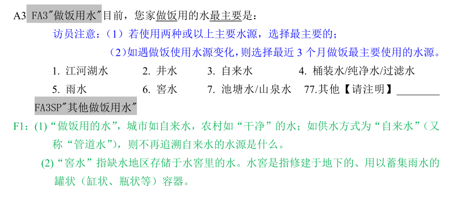
## 2 fa3 做饭用水
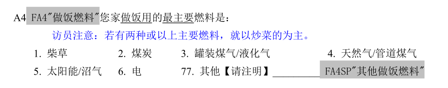
## 3 fa4 做饭燃料
## 4 fa5 通电
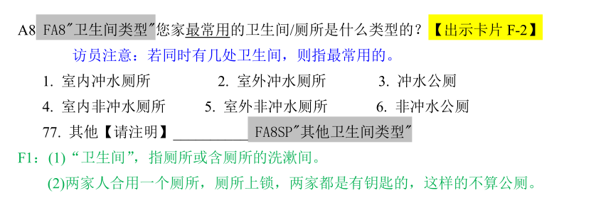
## 5 fa8 卫生间类型
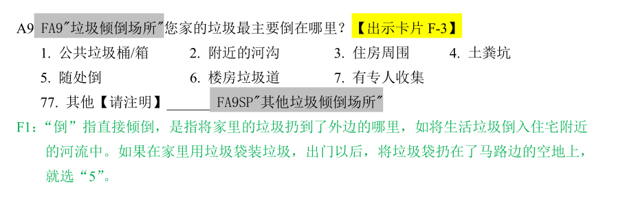
## 6 fa9 垃圾倾倒场所
## 7 fs6_s_1 您家有下列哪些物品-选择1
## 8 fs6_s_2 您家有下列哪些物品-选择2
## 9 fs6_s_3 您家有下列哪些物品-选择3
## 10 fs6_s_4 您家有下列哪些物品-选择4
## # ... with 11 more rowsdf_adult <- cfps2014adult %>%
dplyr::select(
pid, fid14, cfps2012_latest_edu, qp201,
qn12012, qn12013, qn12014, qn1011:qn1017
)
df_adult %>% get_var_label()## # A tibble: 14 x 2
## name label
## <chr> <chr>
## 1 pid 个人ID
## 2 fid14 2014年家庭样本编码
## 3 cfps2012_latest_edu 最近一次调查最高学历
## 4 qp201 健康状况
## 5 qn12012 对自己生活满意度
## 6 qn12013 对自家生活满意度
## 7 qn12014 对自己未来信心程度
## 8 qn1011 因贫富差距而受到不公
## 9 qn1012 因户籍而受到不公
## 10 qn1013 因性别而受到不公
## 11 qn1014 受到政府干部不公
## 12 qn1015 与政府干部发生冲突
## 13 qn1016 到政府办事受到拖延推诿
## 14 qn1017 是否遭政府不合理收费4.3 合并
df_set <- df_famecon %>%
  left_join(df_adult, by = "fid14") # %>%
## Warning: Column `fid14` has different attributes on LHS
## and RHS of join# drop_na()4.4 变量解读
依次对变量解读和规整
colnames(df_set)## [1] "fid14" "fa3"
## [3] "fa4" "fa5"
## [5] "fa8" "fa9"
## [7] "fs6_s_1" "fs6_s_2"
## [9] "fs6_s_3" "fs6_s_4"
## [11] "fs6_s_5" "fs6_s_6"
## [13] "fs6_s_7" "fs6_s_8"
## [15] "fs6_s_9" "fs6_s_10"
## [17] "fs6_s_11" "fs6_s_12"
## [19] "fs6_s_13" "fs6_s_14"
## [21] "fs6_s_15" "pid"
## [23] "cfps2012_latest_edu" "qp201"
## [25] "qn12012" "qn12013"
## [27] "qn12014" "qn1011"
## [29] "qn1012" "qn1013"
## [31] "qn1014" "qn1015"
## [33] "qn1016" "qn1017"df_set %>% get_var_label()## # A tibble: 34 x 2
## name label
## <chr> <chr>
## 1 fid14 2014年家户号
## 2 fa3 做饭用水
## 3 fa4 做饭燃料
## 4 fa5 通电
## 5 fa8 卫生间类型
## 6 fa9 垃圾倾倒场所
## 7 fs6_s_1 您家有下列哪些物品-选择1
## 8 fs6_s_2 您家有下列哪些物品-选择2
## 9 fs6_s_3 您家有下列哪些物品-选择3
## 10 fs6_s_4 您家有下列哪些物品-选择4
## # ... with 24 more rows4.4.1 fid14
df_set %>% count(fid14)## # A tibble: 13,946 x 2
## fid14 n
## <dbl+lbl> <int>
## 1 100051 3
## 2 100125 1
## 3 100160 1
## 4 100286 1
## 5 100376 1
## 6 100435 1
## 7 100453 4
## 8 100551 1
## 9 100569 2
## 10 100724 1
## # ... with 13,936 more rows4.4.2 fa3
df_set %>% count(fa3)## # A tibble: 11 x 2
## fa3 n
## <dbl+lbl> <int>
## 1 -2 1
## 2 -1 4
## 3 1 174
## 4 2 9612
## 5 3 23882
## 6 4 271
## 7 5 111
## 8 6 765
## 9 7 1278
## 10 77 80
## 11 NA 8564.4.3 fa4
df_set %>% count(fa4)## # A tibble: 10 x 2
## fa4 n
## <dbl+lbl> <int>
## 1 -2 1
## 2 -1 3
## 3 1 12021
## 4 2 2286
## 5 3 9779
## 6 4 4335
## 7 5 343
## 8 6 7310
## 9 77 100
## 10 NA 8564.4.4 fa5

df_set %>% count(fa5)## # A tibble: 6 x 2
## fa5 n
## <dbl+lbl> <int>
## 1 -1 1
## 2 1 70
## 3 2 963
## 4 3 13075
## 5 4 22069
## 6 NA 856数据清洗: 无
4.4.5 fa8
df_set %>% count(fa8)## # A tibble: 8 x 2
## fa8 n
## <dbl+lbl> <int>
## 1 1 14717
## 2 2 1707
## 3 3 356
## 4 4 1670
## 5 5 15939
## 6 6 955
## 7 77 834
## 8 NA 8564.4.6 fa9
df_set %>% count(fa9)## # A tibble: 9 x 2
## fa9 n
## <dbl+lbl> <int>
## 1 1 17354
## 2 2 7832
## 3 3 3180
## 4 4 2352
## 5 5 1131
## 6 6 241
## 7 7 3205
## 8 77 883
## 9 NA 8564.4.7 fs6_s_1:fs6_s_15
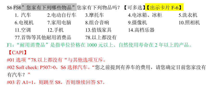
df_set %>% count(fs6_s_1)## # A tibble: 16 x 2
## fs6_s_1 n
## <dbl+lbl> <int>
## 1 1 6184
## 2 2 10081
## 3 3 8931
## 4 4 6865
## 5 5 1290
## 6 6 1986
## 7 7 193
## 8 8 6
## 9 10 8
## 10 11 28
## 11 12 420
## 12 13 5
## 13 14 2
## 14 77 2
## 15 78 177
## 16 NA 8564.4.8 pid
df_set %>% count(pid)## # A tibble: 36,866 x 2
## pid n
## <dbl+lbl> <int>
## 1 100051501 1
## 2 100051502 1
## 3 100453431 1
## 4 101129501 1
## 5 103671501 1
## 6 103788501 1
## 7 103924503 1
## 8 105179433 1
## 9 107624501 1
## 10 108211501 1
## # ... with 36,856 more rows4.4.9 cfps2012_latest_edu
df_set %>% count(cfps2012_latest_edu)## # A tibble: 11 x 2
## cfps2012_latest_edu n
## <dbl+lbl> <int>
## 1 -8 3707
## 2 0 46
## 3 1 9409
## 4 2 7773
## 5 3 9381
## 6 4 4359
## 7 5 1382
## 8 6 763
## 9 7 44
## 10 8 1
## 11 NA 1694.4.10 qp201
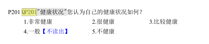
df_set %>% count(qp201)## # A tibble: 9 x 2
## qp201 n
## <dbl+lbl> <int>
## 1 -8 5
## 2 -2 1
## 3 -1 12
## 4 1 5441
## 5 2 7805
## 6 3 12532
## 7 4 5328
## 8 5 5741
## 9 NA 1694.4.11 qn12012:qn12014
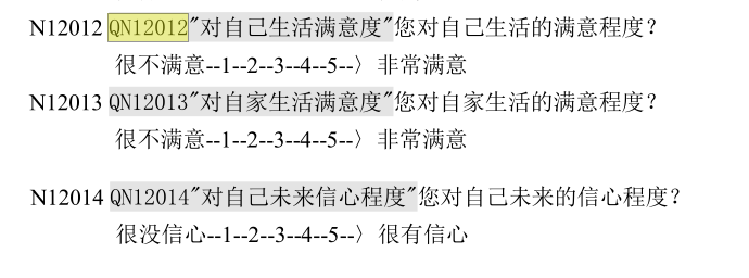
df_set %>% count(qn12012)## # A tibble: 8 x 2
## qn12012 n
## <dbl+lbl> <int>
## 1 -2 4
## 2 -1 29
## 3 1 838
## 4 2 1828
## 5 3 9185
## 6 4 10411
## 7 5 9163
## 8 NA 55764.4.12 qn1011:qn1017
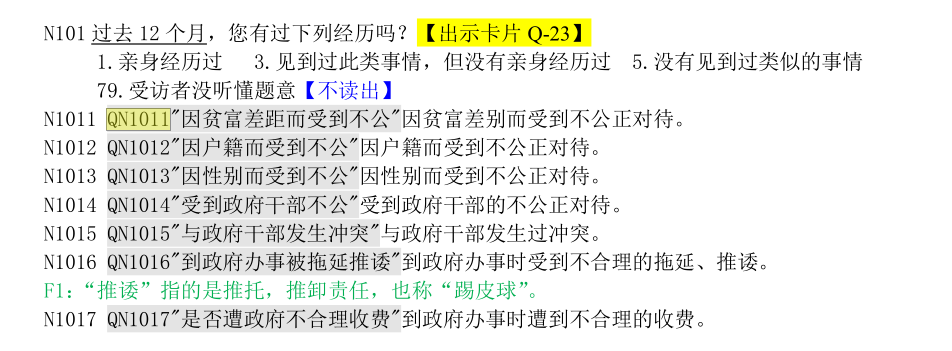
df_set %>% count(qn1011)## # A tibble: 8 x 2
## qn1011 n
## <dbl+lbl> <int>
## 1 -8 4
## 2 -2 5
## 3 -1 15
## 4 1 3691
## 5 3 5103
## 6 5 21914
## 7 79 726
## 8 NA 55764.5 多维度贫困测量
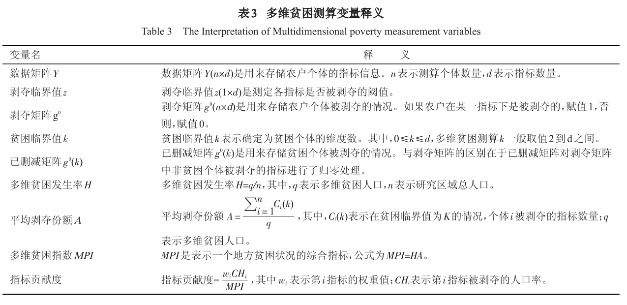
4.6 剥夺矩阵
假定有这样一个数据框
df <- tribble(
  ~id, ~x, ~y, ~z, ~g,
  #--|--|--|--|--
  "a", 13.1, 14, 4, 1,
  "b", 15.2, 7, 5, 0,
  "c", 12.5, 10, 1, 0,
  "d", 20, 11, 3, 1
)
df
## # A tibble: 4 x 5
## id x y z g
## <chr> <dbl> <dbl> <dbl> <dbl>
## 1 a 13.1 14 4 1
## 2 b 15.2 7 5 0
## 3 c 12.5 10 1 0
## 4 d 20 11 3 1设定每个变量的临界值为
cutoffs <- list(
  x = 13,
  y = 12,
  z = 3,
  g = 1
)
剥夺矩阵
get_deprivation_df <- function(df, ..., cutoffs) {
  vars <- rlang::enexprs(...)
  quos <- purrr::map(vars, function(var) {
    rlang::quo(dplyr::if_else(!!var < cutoffs[[rlang::as_name(var)]], 1, 0))
  }) %>%
    purrr::set_names(nm = purrr::map_chr(vars, rlang::as_name))

  df %>%
    dplyr::mutate(!!!quos)
}

g0 <- df %>%
  get_deprivation_df(x, y, z, g, cutoffs = cutoffs)
g0
## # A tibble: 4 x 5
## id x y z g
## <chr> <dbl> <dbl> <dbl> <dbl>
## 1 a 0 0 0 0
## 2 b 0 1 0 1
## 3 c 1 1 1 1
## 4 d 0 1 0 0统计每个人被剥夺了多少, 即每一行中有多个变量是1。
add_deprivations_counting <- function(df) {
  fun <- function(...) sum(c(...) == 1)
  df %>% mutate(n = pmap_dbl(select_if(., is.numeric), fun))
}

g0_k <- g0 %>% add_deprivations_counting()
g0_k
## # A tibble: 4 x 6
## id x y z g n
## <chr> <dbl> <dbl> <dbl> <dbl> <dbl>
## 1 a 0 0 0 0 0
## 2 b 0 1 0 1 2
## 3 c 1 1 1 1 4
## 4 d 0 1 0 0 1得到了剥夺矩阵,下面进行的是贫困人口识别。
4.6.1 识别方法一:统计剥夺变量个数
再给定一个k值,如果每个人剥夺次数小于k值,说明不贫穷,那么这个人所在行全部归零。 没被清零的,说明是贫穷的
censor_aggregation <- function(df, k) {
  fun <- function(...) sum(c(...) == 1)
  df %>%
    nest(-id, -n) %>%
    mutate(data = if_else(
      n == k, # Censor data of nonpoor
      map(data, function(x) mutate_all(x, funs(replace(., TRUE, 0)))),
      data
    )) %>%
    tidyr::unnest() %>%
    dplyr::select(-n) %>%
    mutate(n = pmap_dbl(select_if(., is.numeric), fun))
}

g0_k1 <- g0_k %>% censor_aggregation(k = 1)
g0_k1
## # A tibble: 4 x 6
## id x y z g n
## <chr> <dbl> <dbl> <dbl> <dbl> <dbl>
## 1 a 0 0 0 0 0
## 2 b 0 1 0 1 2
## 3 c 1 1 1 1 4
## 4 d 0 0 0 0 0根据上面识别出来的贫穷人口,计算一些比率
Headcount_Ratio <- function(df) {
  d <- nrow(df)
  q <- df %>% summarise(num_nopoor = sum(n != 0)) %>% pull()
  H <- q / d

  return(H)
}

average_deprivation_share <- function(df) {
  d <- nrow(df)
  q <- df %>% summarise(num_nopoor = sum(n != 0)) %>% pull()
  A <- df %>%
    mutate(ck_d = n / d) %>%
    summarise(sum_sk_d = sum(ck_d) / q) %>%
    pull()

  return(A)
}
g0_k1 %>% Headcount_Ratio()## [1] 0.5g0_k1 %>% average_deprivation_share()## [1] 0.754.6.2 识别方法二:赋予变量权重再统计
这里不再是数每行有多少个1,而是对每个变量赋予权重,求得贫困系数(或者叫贫困概率)。这个过程 也可以用tidyverse的办法
weights <- c(
  x = 0.25,
  y = 0.25,
  z = 0.25,
  g = 0.25
)

weighted_sum <- function(.data, weights) {
  ab <- .data %>%
    gather(var, val, x:g) %>%
    mutate(x_weight = val * weights[var]) %>%
    group_by(id) %>%
    summarise(sum_weight = sum(x_weight))

  .data %>% left_join(ab)
}


g0 %>% weighted_sum(weights)
## Joining, by = "id"## # A tibble: 4 x 6
## id x y z g sum_weight
## <chr> <dbl> <dbl> <dbl> <dbl> <dbl>
## 1 a 0 0 0 0 0
## 2 b 0 1 0 1 0.5
## 3 c 1 1 1 1 1
## 4 d 0 1 0 0 0.25或者
fun <- function(...) {weighted.mean(..., weights)}
g0 %>% mutate(wt_sum = pmap_dbl(select_if(., is.numeric), lift_vd(fun)))
## # A tibble: 4 x 6
## id x y z g wt_sum
## <chr> <dbl> <dbl> <dbl> <dbl> <dbl>
## 1 a 0 0 0 0 0
## 2 b 0 1 0 1 0.5
## 3 c 1 1 1 1 1
## 4 d 0 1 0 0 0.254.7 变量赋权重再统计(一站式代码)
给出每个变量的临界值,得到剥夺矩阵,然后再对每个变量赋予权重,求得贫困系数(或者叫贫困概率),根据贫困系数,我们识别贫困人口。事实上,这两步可以合并成一步来完成。
cutoffs <- list(
  x = 13,
  y = 12,
  z = 3,
  g = 1
)

weights <- c(
  x = 0.25,
  y = 0.25,
  z = 0.25,
  g = 0.25
)

df_wt <- df %>%
  gather(var, val, x:g) %>%
  mutate(below_cutoff = as.integer(val < cutoffs[var])) %>%
  mutate(weighted_point = below_cutoff * weights[var]) %>%
  group_by(id) %>%
  summarise(weighted_sum = sum(weighted_point))

df %>% left_join(df_wt)
## Joining, by = "id"## # A tibble: 4 x 6
## id x y z g weighted_sum
## <chr> <dbl> <dbl> <dbl> <dbl> <dbl>
## 1 a 13.1 14 4 1 0
## 2 b 15.2 7 5 0 0.5
## 3 c 12.5 10 1 0 1
## 4 d 20 11 3 1 0.25或者写出子函数的形式,一劳永逸
cutoffs <- c(
  x = 13,
  y = 12,
  z = 3,
  g = 1
)

weights <- c(
  x = 0.25,
  y = 0.25,
  z = 0.25,
  g = 0.25
)

get_weightedSum_df <- function(.data, cutoffs, weights) {
  ab <- .data %>%
    gather(var, val, x:g) %>%
    mutate(below_cutoff = as.integer(val < cutoffs[var])) %>%
    mutate(weighted_point = below_cutoff * weights[var]) %>%
    group_by(id) %>%
    summarise(weightSum = sum(weighted_point))

  .data %>% left_join(ab)
}


df %>% get_weightedSum_df(cutoffs, weights)
## # A tibble: 4 x 6
## id x y z g weightSum
## <chr> <dbl> <dbl> <dbl> <dbl> <dbl>
## 1 a 13.1 14 4 1 0
## 2 b 15.2 7 5 0 0.5
## 3 c 12.5 10 1 0 1
## 4 d 20 11 3 1 0.25