Chapter 8 Conditional manatees

8.1 Building an interaction

\(R\) = ruggedness, \(G\) = GDP, \(C\) = continent, \(U\) = unobserved variables.

library(dagitty)
library(rethinking)
dag_8.1 <- dagitty("dag{
                   R -> G
                   C -> G
                   U -> G
                   U -> R
                   }")
coordinates(dag_8.1) <- list(y = c(R = 0, G = 0, C = 0, U = 1),
                             x = c(R = 0, G = 1, U = 1, C = 2))
drawdag(dag_8.1)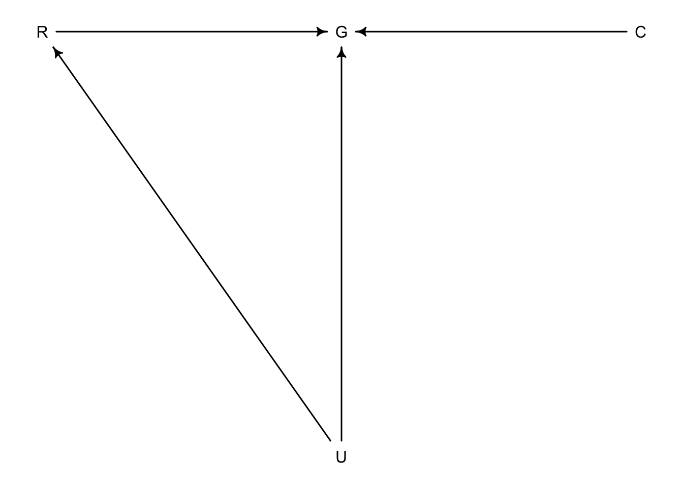

\(G = f(R,C)\)

8.1.1 Making a rugged model

library(rethinking)
data(rugged)
d <- rugged

#log transform GDP
d$log_gdp <- log(d$rgdppc_2000)

#only include countries with GDP data
dd <- d[complete.cases(d$rgdppc_2000),]

#rescale variables
dd$log_gdp_std <- (dd$log_gdp) / mean(dd$log_gdp) # values of 1 is average
dd$rugged_std <- (dd$rugged) / max(dd$rugged) # values range from 0 to max ruggedness (1)

Basic model \[\text{log}(y_{i}) \sim \text{Normal}(\mu_{i}, \sigma)\\ \mu_{i} = \alpha + \beta(r_{i} - \overline{r})\\ \alpha \sim \text{Normal}|(1,1)\\ \beta \sim \text{Normal}(0, 1)\\ \sigma \sim \text{Exponential}(1)\]

In R:

m8.1 <- quap(
  alist(
    log_gdp_std ~ dnorm(mu, sigma),
    mu <- a + b*(rugged_std - 0.215),
    a ~ dnorm(1, 1),
    b ~ dnorm(0, 1),
    sigma ~ dexp(1)
  ), data = dd
)

Sample priors:

set.seed(11)
prior <- extract.prior(m8.1)

#set plot
plot(NULL, xlim=c(0,1), ylim=c(0.5, 1.5), xlab = "ruggedness", ylab = "log GDP")
abline(h=min(dd$log_gdp_std), lty = 2)
abline(h=max(dd$log_gdp_std), lty = 2)

#draw lines from prior
rugged_seq <- seq(from = -0.1, to = 1.1, length.out=30)
mu <- link(m8.1, post = prior, data = data.frame(rugged_std=rugged_seq))
for(i in 1:50){
  lines(rugged_seq, mu[i,], col=col.alpha('black',0.3))
  }

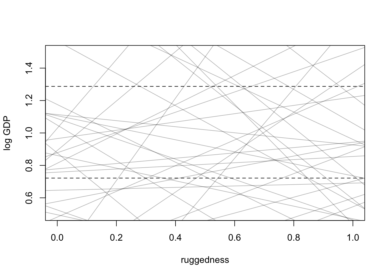
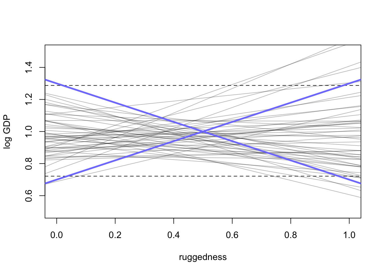
\(\alpha\) is too wild. intercept should be somewhere around where the mean of ruggedness hits 1 on the log GDP scale so adjust to Normal(1, 0.1).

\(\beta\) is also out of control. we need something (positive or negative) that spans the difference between the dashed lines

Slope should be \(\pm 0.6\) which is the differece between the maximum and minimum values of GDP

max(dd$log_gdp_std) - min(dd$log_gdp_std)

## [1] 0.5658058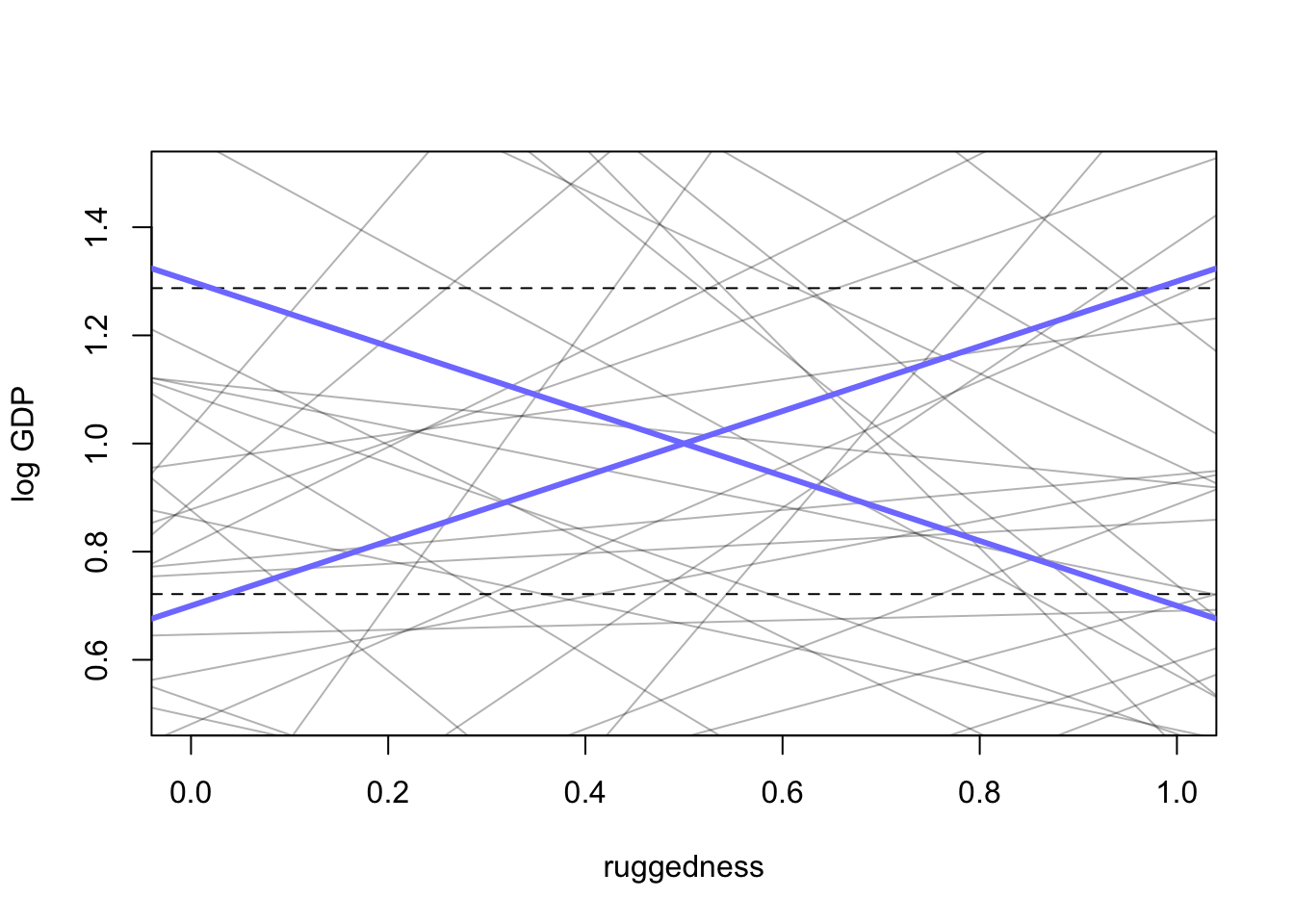

#proportion of slopes greater than 0.6
sum(abs(prior$b) > 0.6) / length(prior$b)

## [1] 0.54

Let’s fix the model

m8.1 <- quap(
  alist(
    log_gdp_std ~dnorm(mu,sigma),
    mu <-a+b*(rugged_std-0.215),
    a ~dnorm(1,0.1),
    b ~dnorm(0,0.3),
    sigma ~dexp(1)
  ), data = dd
)

precis(m8.1)

##              mean          sd        5.5%      94.5%
## a     0.999998578 0.010412457  0.98335746 1.01663970
## b     0.001994904 0.054795958 -0.08557962 0.08956943
## sigma 0.136503830 0.007397023  0.12468196 0.14832570

No association seen yet

8.1.2 Adding an indicator isn’t enough

Update \(\mu\)

\[\mu_{i} = \alpha_{CID[i]} + \beta(r_{i} - \overline{r})\]

#make an index variable for Africa (1) and other continents (2)
dd$cid <- ifelse(dd$cont_africa == 1, 1, 2)

Now update the model

m8.2 <- quap(
  alist(
    log_gdp_std ~ dnorm(mu, sigma),
    mu <-a[cid] + b * (rugged_std - 0.215),
    a[cid] ~ dnorm(1, 0.1),
    b ~ dnorm(0, 0.3),
    sigma ~dexp(1)
  ), data = dd
)

compare(m8.1, m8.2)

##           WAIC       SE    dWAIC      dSE    pWAIC       weight
## m8.2 -252.1508 15.25508  0.00000       NA 4.291725 1.000000e+00
## m8.1 -188.9664 13.28913 63.18439 15.11018 2.574284 1.904075e-14

precis(m8.2, depth = 2)

##              mean          sd       5.5%      94.5%
## a[1]   0.88040848 0.015938408  0.8549358 0.90588113
## a[2]   1.04916209 0.010186473  1.0328821 1.06544204
## b     -0.04651791 0.045690786 -0.1195406 0.02650479
## sigma  0.11239762 0.006092464  0.1026607 0.12213455

post <- extract.samples(m8.2)
diff_a1_a2 <- post$a[,1] - post$a[,2]
PI(diff_a1_a2)

##         5%        94% 
## -0.1988472 -0.1384092

rugged.seq <- seq(from = -0.1, to = 1.1, length.out = 30)
mu.NotAfrica <- link(m8.2, data = data.frame(cid=2, rugged_std=rugged.seq))
mu.Africa <- link(m8.2, data = data.frame(cid = 1, rugged_std = rugged.seq))
mu.NotAfrica_mu <- apply(mu.NotAfrica, 2, mean)
mu.NotAfrica_ci <- apply(mu.NotAfrica, 2, PI, prob = 0.97)
mu.Africa_mu <- apply(mu.Africa, 2, mean)
mu.Africa_ci <- apply(mu.Africa, 2, PI)

plot(NULL, xlim=c(0,1), ylim=c(0.5, 1.5), xlab = "ruggedness", ylab = "log GDP")
points(dd$rugged_std, dd$log_gdp_std, col = dd$cid, pch = 16)
lines(rugged.seq, mu.Africa_mu, lwd = 2, col = 1)
shade(mu.Africa_ci, rugged.seq)
lines(rugged.seq, mu.NotAfrica_mu, lwd = 2, col = 2)
shade(mu.NotAfrica_ci, rugged.seq, col = col.alpha(2, 0.3))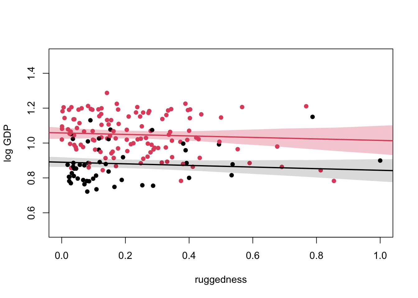

8.1.3 Adding an interaction does work

\[\mu_{i} = \alpha_{CID[i]} + \beta_{CID[i]}(r_{i} - \overline{r})\]

m8.3 <- quap(
  alist(
     log_gdp_std ~ dnorm(mu, sigma),
    mu <-a[cid] + b[cid] * (rugged_std - 0.215),
    a[cid] ~ dnorm(1, 0.1),
    b[cid] ~ dnorm(0, 0.3),
    sigma ~dexp(1)
  ), data = dd
)

precis(m8.3, depth = 2)

##             mean          sd        5.5%       94.5%
## a[1]   0.8865632 0.015675727  0.86151037  0.91161605
## a[2]   1.0505709 0.009936627  1.03469025  1.06645155
## b[1]   0.1325019 0.074204597  0.01390861  0.25109517
## b[2]  -0.1425818 0.054749512 -0.23008206 -0.05508147
## sigma  0.1094944 0.005935331  0.10000855  0.11898016

compare(m8.1, m8.2, m8.3, func=PSIS)

## Some Pareto k values are high (>0.5). Set pointwise=TRUE to inspect individual points.

##           PSIS       SE     dPSIS       dSE    pPSIS       weight
## m8.3 -258.8749 15.35435  0.000000        NA 5.314384 9.688047e-01
## m8.2 -252.0033 15.30167  6.871589  6.936621 4.354277 3.119533e-02
## m8.1 -188.4136 13.40307 70.461243 15.674795 2.856543 4.850334e-16

plot(PSIS(m8.3, pointwise = TRUE)$k)

## Some Pareto k values are high (>0.5). Set pointwise=TRUE to inspect individual points.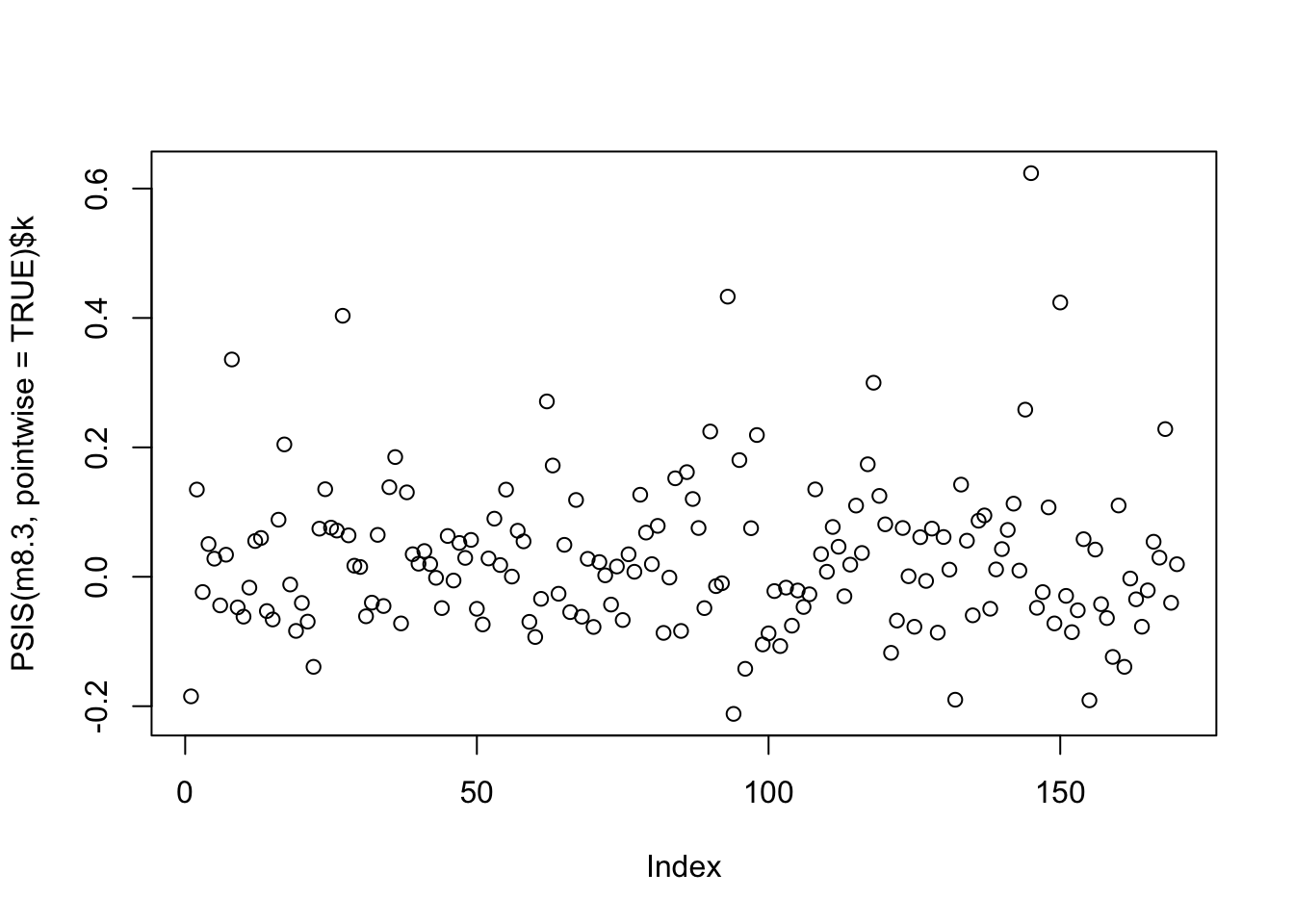

8.1.4 Plotting the interaction

par(mfrow=c(1,2))
# plot Africa - cid = 1
d.A1 <-dd[dd$cid == 1,]
plot(d.A1$rugged_std, d.A1$log_gdp_std, pch=16, col=rangi2,
xlab="ruggedness (standardized)",ylab="log GDP (as proportion of mean)",
xlim=c(0,1) )
mu <-link(m8.3,data=data.frame(cid=1,rugged_std=rugged_seq))
mu_mean <-apply(mu,2,mean)
mu_ci <-apply(mu,2,PI,prob=0.97)
lines( rugged_seq,mu_mean,lwd=2)
shade( mu_ci,rugged_seq,col=col.alpha(rangi2,0.3))
mtext("African nations")
# plotnon-Africa-cid=2
d.A0 <-dd[dd$cid==2,]
plot( d.A0$rugged_std,d.A0$log_gdp_std,pch=1,col="black",
xlab="ruggedness (standardized)",ylab="logGDP(asproportionofmean)",
xlim=c(0,1) )
mu <-link(m8.3,data=data.frame(cid=2,rugged_std=rugged_seq))
mu_mean <-apply(mu,2,mean)
mu_ci <-apply(mu,2,PI,prob=0.97)
lines( rugged_seq,mu_mean,lwd=2)
shade( mu_ci,rugged_seq)
mtext("Non-African nations")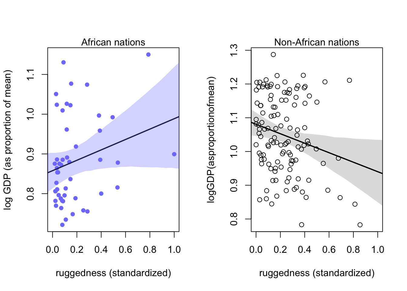

8.2 Symmetry of interactions

You can break an interaction into 2 identical phrasings
1. GDP ~ ruggedness depending on Africa
2. Africa ~ GDP depending on rugedness

\[\mu_{i} = (2 - CID_{i})(\alpha_{1} + \beta_{1}(r_{i} - \overline{r})) + (CID_{i} - 1)(\alpha_{2} + \beta_{2}(r_{i} - \overline{r}))\]

rugged_seq <- seq(from = -0.2, to = 1.2, length.out = 30)
muA <- link(m8.3, data=data.frame(cid=1, rugged_std=rugged_seq))
muN <- link(m8.3, data=data.frame(cid=2, rugged_std=rugged_seq))
delta <- muA - muN


mu.delta <- apply(delta, 2, mean)
PI.delta <- apply(delta, 2, PI)

plot(x=rugged_seq, type = 'n', xlim = c(0,1), ylim = c(-0.3, 0.2),
     xlab = 'ruggedness (std)', ylab = 'expected difference log GDP')
shade(PI.delta, rugged_seq, col='grey')
abline(h = 0, lty = 2)
text(x = 0.2, y = 0, label = "Africa higher GDP\nAfrica lower GDP")
lines(rugged_seq, mu.delta)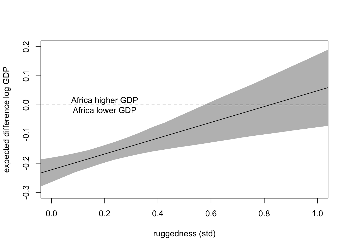

At high ruggedness, being in Africa gives higher than expected GDP.

8.3 Continuous interactions

8.3.1 A winter flower

data(tulips)
d <- tulips
str(d)

## 'data.frame':    27 obs. of  4 variables:
##  $ bed   : Factor w/ 3 levels "a","b","c": 1 1 1 1 1 1 1 1 1 2 ...
##  $ water : int  1 1 1 2 2 2 3 3 3 1 ...
##  $ shade : int  1 2 3 1 2 3 1 2 3 1 ...
##  $ blooms: num  0 0 111 183.5 59.2 ...

8.3.2 the models

Water and Shade work together to create Blooms; \(W \rightarrow B \leftarrow S ; B = f(W,S)\)

1. water
   \[\beta_{i} \sim \text{Normal}(\mu_{i}, \sigma)\\ \mu_{i} = \alpha + \beta_{W}(W_{i} - \overline{W})\\ \alpha \sim \text{Normal}(0.5,1)\\ \beta_{W} \sim \text{Normal}(0,1)\\ \sigma \sim \text{Exponential}(1)\]
2. shade
   \[\beta_{i} \sim \text{Normal}(\mu_{i}, \sigma)\\ \mu_{i} = \alpha + \beta_{S}(S_{i} - \overline{S})\\ \alpha \sim \text{Normal}(0.5,1)\\ \beta_{S} \sim \text{Normal}(0,1)\\ \sigma \sim \text{Exponential}(1)\]
3. water + shade
   \[\beta_{i} \sim \text{Normal}(\mu_{i}, \sigma)\\ \mu_{i} = \alpha + \beta_{W}(W_{i} - \overline{W}) + \beta_{S}(S_{i} - \overline{S})\\ \alpha \sim \text{Normal}(0.5,1)\\ \beta_{W} \sim \text{Normal}(0,1)\\ \beta_{S} \sim \text{Normal}(0,1)\\ \sigma \sim \text{Exponential}(1)\]
4. water * shade
   $$$$

#center predictors and scale outcome
d$blooms_std <- d$blooms / max(d$blooms)
d$water_cent <- d$water - mean(d$water)
d$shade_cent <- d$shade - mean(d$shade)

The \(\alpha\) prior is likely too broad. We need it to be between 0 and 1. How much is outside that?

a <- rnorm(1e4, 0.5, 1); sum(a < 0 | a > 1) / length(a)

## [1] 0.623

Let’s tighten it

a <- rnorm(1e4, 0.5, 0.25); sum(a < 0 | a > 1) / length(a)

## [1] 0.047

range of water and shade are each 2 units. range of blooms is one unit. max slopes = 2/1 (0.5) so we can set the prior to 0 with 0.25 sd to get values ranging from -0.5 to 0.5.

#water
m8.4a <- quap(
  alist(
    blooms_std ~ dnorm(mu, sigma),
    mu <- a + bw*water_cent,
    a ~ dnorm(0.5,0.25),
    bw ~ dnorm(0, 0.25),
    sigma ~ dexp(1)
  ), data = d
)

#shade
m8.4b <- quap(
  alist(
    blooms_std ~ dnorm(mu, sigma),
    mu <- a + bs*shade_cent,
    a ~ dnorm(0.5,0.25),
    bs ~ dnorm(0, 0.25),
    sigma ~ dexp(1)
  ), data = d
)

# water + shade
m8.4c <- quap(
  alist(
    blooms_std ~ dnorm(mu, sigma),
    mu <- a + bw*water_cent + bs*shade_cent,
    a ~ dnorm(0.5,0.25),
    bw ~ dnorm(0, 0.25),
    bs ~ dnorm(0, 0.25),
    sigma ~ dexp(1)
  ), data = d
)

#water * shade
m8.4d <- quap(
  alist(
    blooms_std ~ dnorm(mu, sigma),
    mu <- a + bw*water_cent + bs*shade_cent + bws*water_cent*shade_cent,
    a ~ dnorm(0.5,0.25),
    bw ~ dnorm(0, 0.25),
    bs ~ dnorm(0, 0.25),
    bws ~ dnorm(0, 0.25),
    sigma ~ dexp(1)
  ), data = d
)

prior simulations

set.seed(11)
prior_a <- extract.prior(m8.4a) #water
prior_b <- extract.prior(m8.4b) #shade
prior_c <- extract.prior(m8.4c) #water + shade
prior_d <- extract.prior(m8.4d) #water * shade


#set plot
plot(NULL, xlim=c(0,2), ylim=c(0, 1.25), xlab = "Water / shade", ylab = "blooms")
abline(h=min(d$blooms_std), lty = 2)
abline(h=max(d$blooms_std), lty = 2)

#draw lines from prior
water_seq <- seq(from = -1.1, to = 1.1, length.out=30)
shade_seq <- seq(from = -1.1, to = 1.1, length.out=30)

mu_a <- link(m8.4a, post = prior_a, data = data.frame(water_cent=water_seq))
mu_b <- link(m8.4b, post = prior_b, data = data.frame(shade_cent=shade_seq))
mu_c <- link(m8.4c, post = prior_c, data = data.frame(water_cent=water_seq, shade_cent=shade_seq))
mu_d <- link(m8.4d, post = prior_d, data = data.frame(water_cent=water_seq, shade_cent=shade_seq))

#set plot
plot(NULL, xlim=c(-1,1), ylim=c(0, 1.25), xlab = "Water / shade (centered)", ylab = "blooms (std)")
abline(h=min(d$blooms_std), lty = 2)
abline(h=max(d$blooms_std), lty = 2)


for(i in 1:50){
  lines(water_seq, mu_a[i,], col=col.alpha('blue',0.3))
  }

for(i in 1:50){
  lines(water_seq, mu_b[i,], col=col.alpha('black',0.3))
}
for(i in 1:50){
  lines(water_seq, mu_c[i,], col=col.alpha('green',0.3))
}

for(i in 1:50){
  lines(water_seq, mu_d[i,], col=col.alpha('red',0.3))
  }

text(x = -0.75, y = 1.2, label = "Water", col = "blue")
text(x = -0.45, y = 1.2, label = "Shade", col = "black")
text(x = 0, y = 1.2, label = "Water + Shade", col = "green")
text(x = 0.5, y = 1.2, label = "Water * Shade", col = 'red')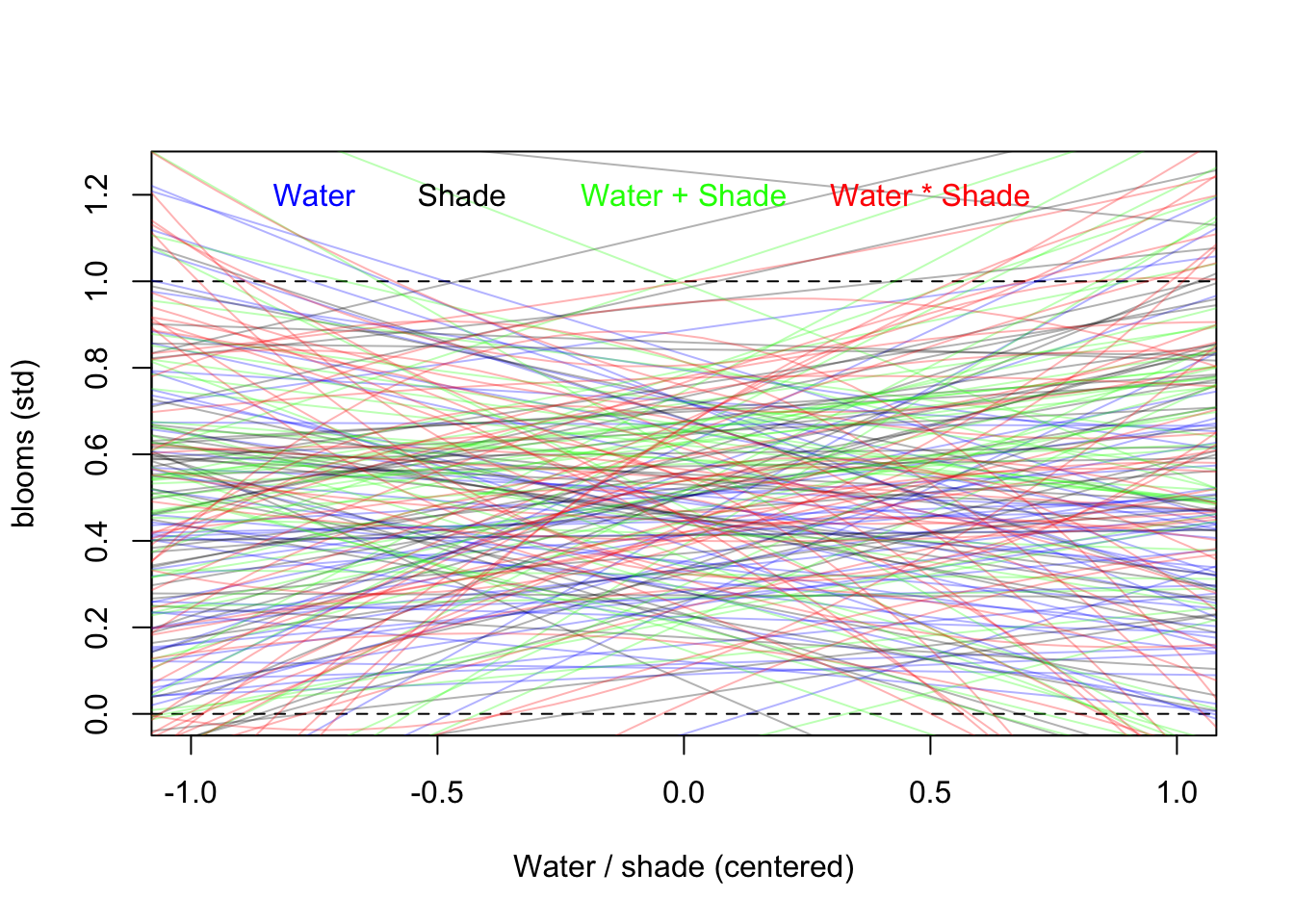

precis(m8.4a)

##            mean         sd      5.5%     94.5%
## a     0.3594883 0.03502089 0.3035181 0.4154584
## bw    0.2034854 0.04270338 0.1352371 0.2717336
## sigma 0.1837433 0.02489828 0.1439510 0.2235355

precis(m8.4b)

##             mean         sd       5.5%       94.5%
## a      0.3611171 0.04403635  0.2907385  0.43149566
## bs    -0.1097643 0.05351857 -0.1952973 -0.02423127
## sigma  0.2323701 0.03143809  0.1821260  0.28261427

precis(m8.4c)

##             mean         sd       5.5%       94.5%
## a      0.3587452 0.03022116  0.3104459  0.40704441
## bw     0.2050352 0.03689240  0.1460741  0.26399641
## bs    -0.1125324 0.03687853 -0.1714714 -0.05359337
## sigma  0.1581668 0.02144796  0.1238888  0.19244481

precis(m8.4d)

##             mean         sd        5.5%       94.5%
## a      0.3579980 0.02391747  0.31977332  0.39622278
## bw     0.2067288 0.02923282  0.16000910  0.25344849
## bs    -0.1134595 0.02922579 -0.16016795 -0.06675103
## bws   -0.1431791 0.03567746 -0.20019860 -0.08615967
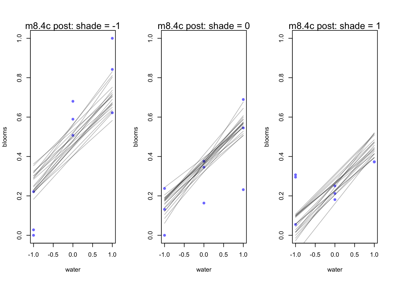
## sigma  0.1248375 0.01693790  0.09776742  0.15190750

8.3.3 Plotting posterior predictions

par(mfrow = c(1,3))
for (s in -1:1){
  idx <- d[d$shade_cent == s,]
  plot(x = idx$water_cent, y = idx$blooms_std, xlim = c(-1,1), ylim = c(0,1),
       xlab = "water", ylab = "blooms", pch = 16, col = rangi2)
  mu <- link(m8.4c, data = data.frame(shade_cent=s, water_cent = -1:1))
  for(i in 1:20){
    lines(-1:1, mu[i,], col = col.alpha('black',0.3))
  }
   mtext(concat("m8.4c post: shade = ", s))
}

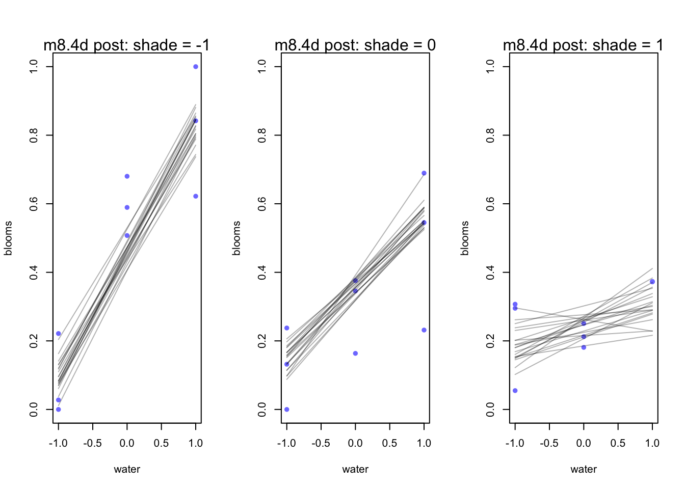
par(mfrow = c(1,3))
for (s in -1:1){
  idx <- d[d$shade_cent == s,]
  plot(x = idx$water_cent, y = idx$blooms_std, xlim = c(-1,1), ylim = c(0,1),
       xlab = "water", ylab = "blooms", pch = 16, col = rangi2)
  mu <- link(m8.4d, data = data.frame(shade_cent=s, water_cent = -1:1))
  for(i in 1:20){
    lines(-1:1, mu[i,], col = col.alpha('black',0.3))
  }
   mtext(concat("m8.4d post: shade = ", s))
}

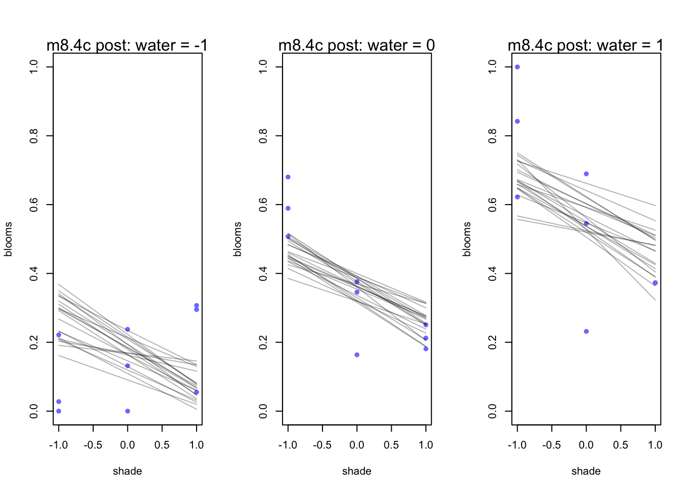
par(mfrow = c(1,3))
for (s in -1:1){
  idx <- d[d$water_cent == s,]
  plot(x = idx$shade_cent, y = idx$blooms_std, xlim = c(-1,1), ylim = c(0,1),
       xlab = "shade", ylab = "blooms", pch = 16, col = rangi2)
  mu <- link(m8.4c, data = data.frame(water_cent=s, shade_cent = -1:1))
  for(i in 1:20){
    lines(-1:1, mu[i,], col = col.alpha('black',0.3))
  }
  mtext(concat("m8.4c post: water = ", s))
}

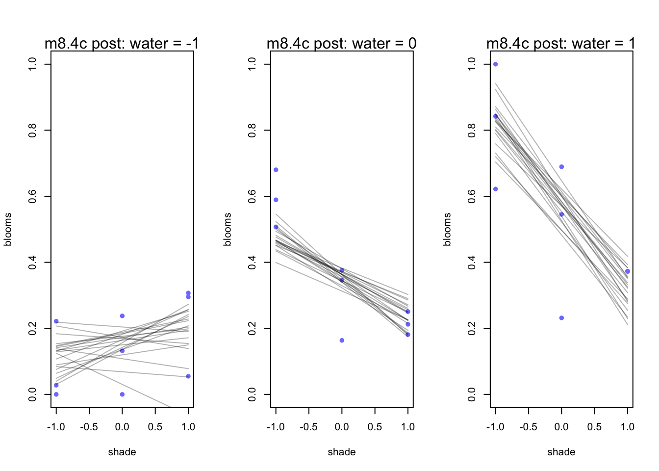
par(mfrow = c(1,3))
for (s in -1:1){
  idx <- d[d$water_cent == s,]
  plot(x = idx$shade_cent, y = idx$blooms_std, xlim = c(-1,1), ylim = c(0,1),
       xlab = "shade", ylab = "blooms", pch = 16, col = rangi2)
  mu <- link(m8.4d, data = data.frame(water_cent=s, shade_cent = -1:1))
  for(i in 1:20){
    lines(-1:1, mu[i,], col = col.alpha('black',0.3))
  }
  mtext(concat("m8.4c post: water = ", s))
}

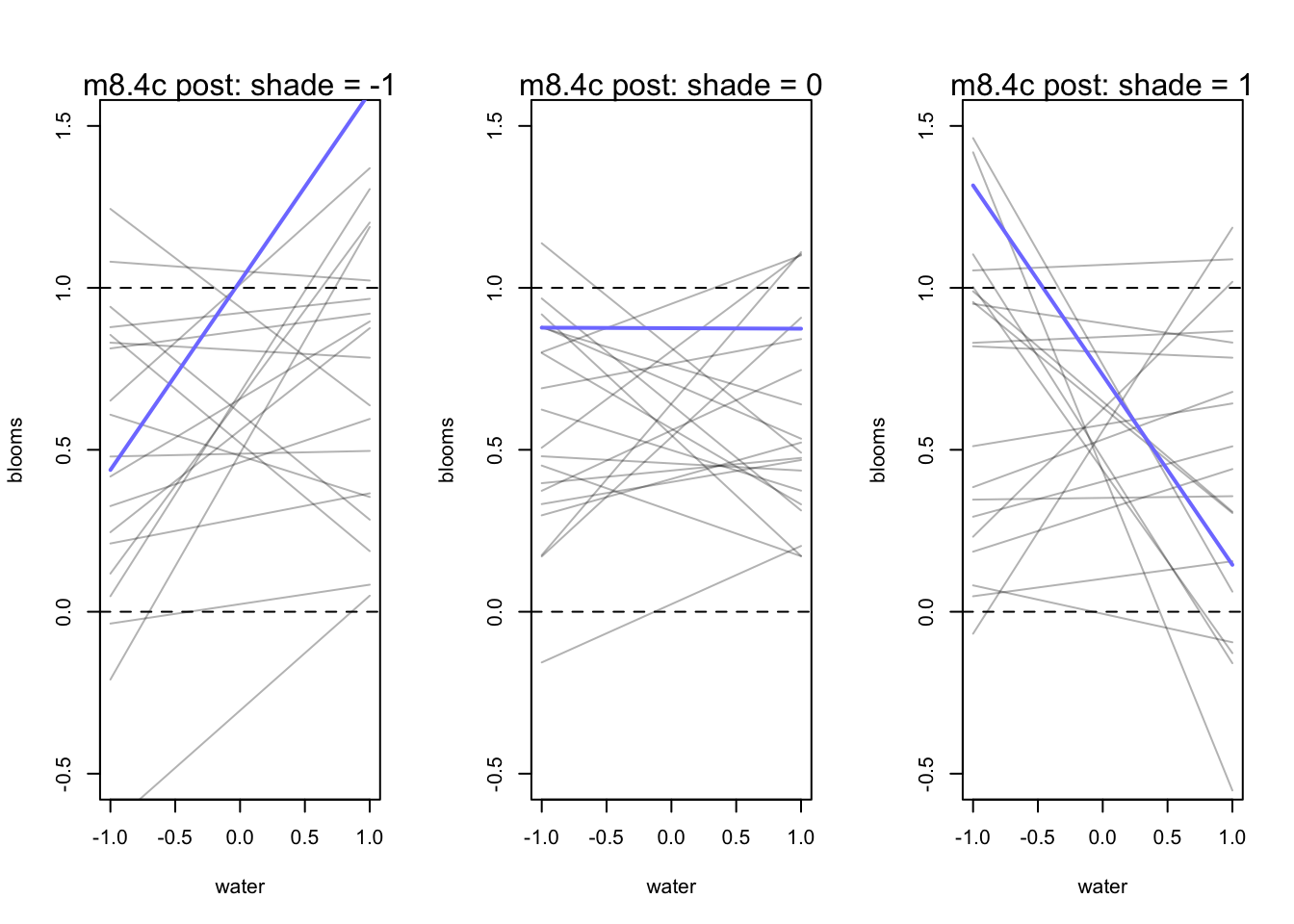
8.3.4 Plotting prior predictions

par(mfrow = c(1,3))
for (s in -1:1){
  idx <- d[d$shade_cent == s,]
  plot(x = idx$water_cent, y = idx$blooms_std, type = 'n', xlim = c(-1,1), ylim = c(-0.5,1.5),
       xlab = "water", ylab = "blooms")
  mu <- link(m8.4c, post = prior_c, data = data.frame(shade_cent=s, water_cent = -1:1))
  for(i in 1:20){
    lines(-1:1, mu[i,], col = col.alpha('black',0.3))
  }
  lines(-1:1, mu[11,], lwd = 2, col = rangi2)
  abline(h = 0, lty = 2)
  abline(h = 1, lty = 2)
  mtext(concat("m8.4c post: shade = ", s))
}

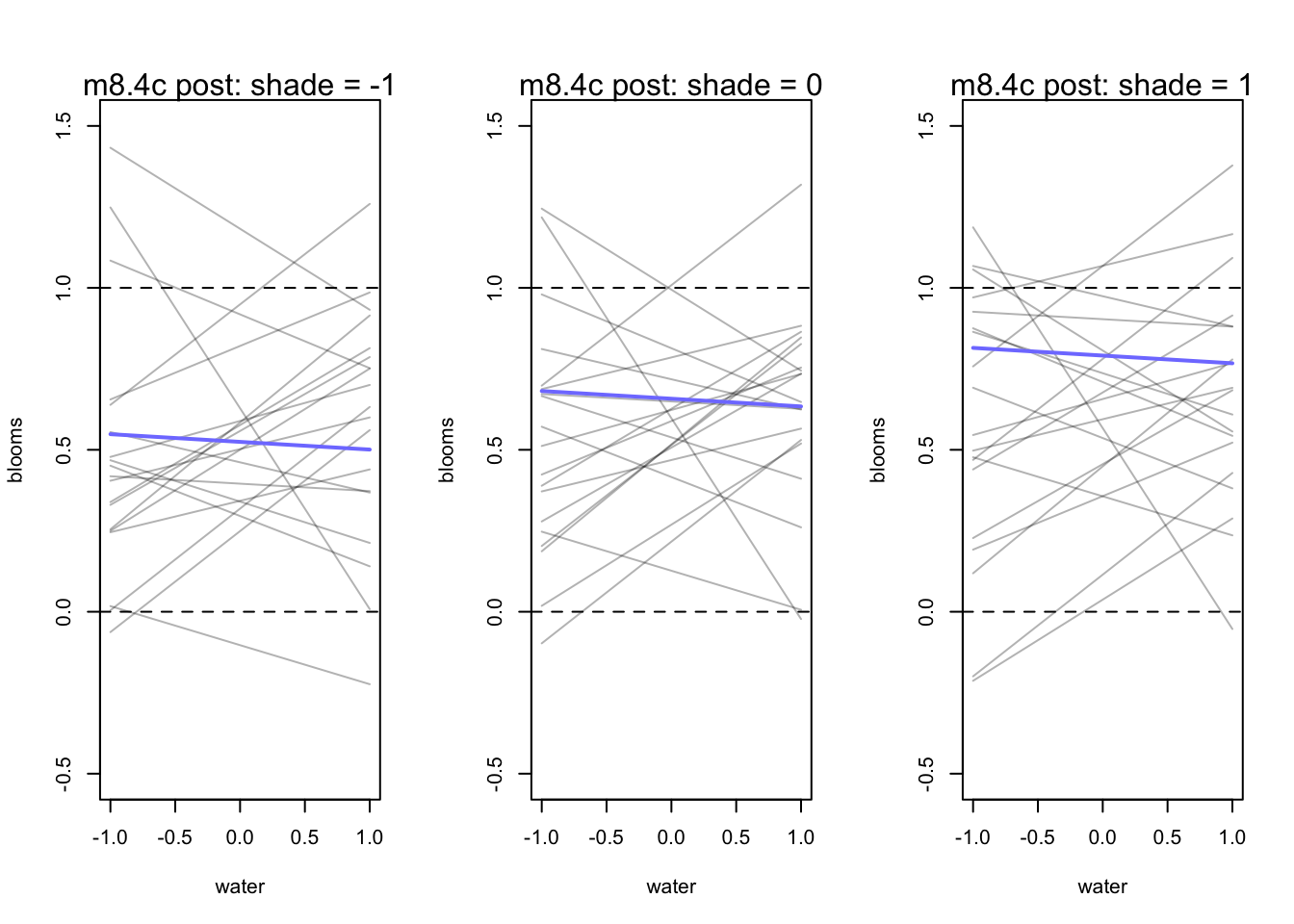
par(mfrow = c(1,3))
for (s in -1:1){
  idx <- d[d$shade_cent == s,]
  plot(x = idx$water_cent, y = idx$blooms_std, type = 'n', xlim = c(-1,1), ylim = c(-0.5,1.5),
       xlab = "water", ylab = "blooms")
  mu <- link(m8.4d, post = prior_d, data = data.frame(shade_cent=s, water_cent = -1:1))
  for(i in 1:20){
    lines(-1:1, mu[i,], col = col.alpha('black',0.3))
  }
  lines(-1:1, mu[11,], lwd = 2, col = rangi2)
  abline(h = 0, lty = 2)
  abline(h = 1, lty = 2)
  mtext(concat("m8.4c post: shade = ", s))
}

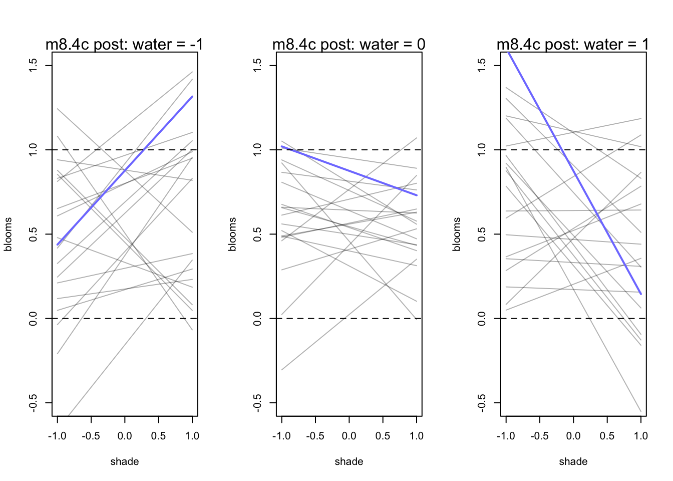
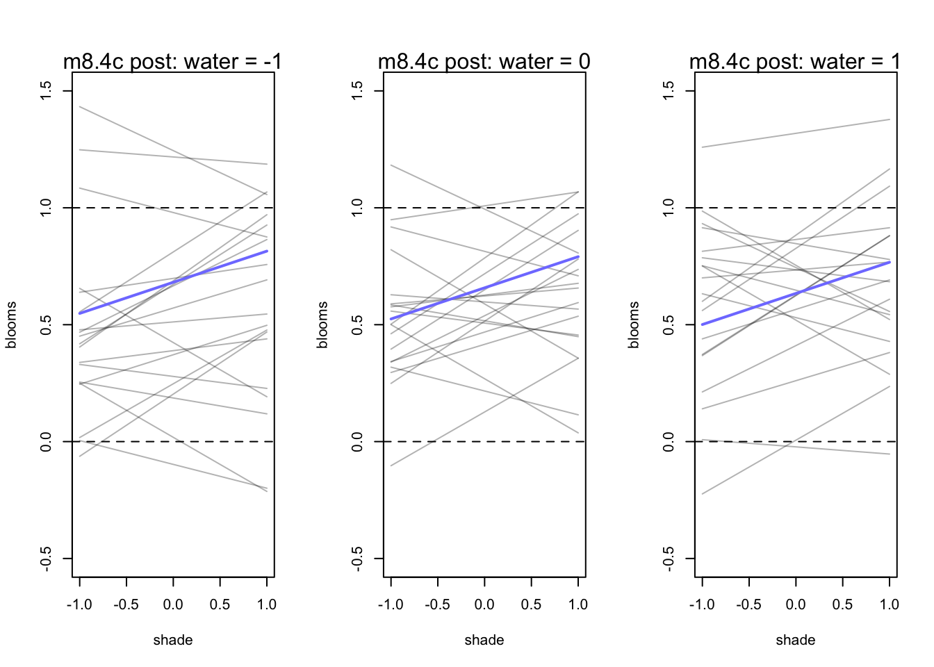
par(mfrow = c(1,3))
for (s in -1:1){
  idx <- d[d$water_cent == s,]
  plot(x = idx$shade_cent, y = idx$blooms_std, type = 'n', xlim = c(-1,1), ylim = c(-0.5,1.5),
       xlab = "shade", ylab = "blooms")
  mu <- link(m8.4c, post = prior_c, data = data.frame(water_cent=s, shade_cent = -1:1))
  for(i in 1:20){
    lines(-1:1, mu[i,], col = col.alpha('black',0.3))
  }
  lines(-1:1, mu[11,], lwd = 2, col = rangi2)
  abline(h = 0, lty = 2)
  abline(h = 1, lty = 2)
  mtext(concat("m8.4c post: water = ", s))
}

par(mfrow = c(1,3))
for (s in -1:1){
  idx <- d[d$water_cent == s,]
  plot(x = idx$shade_cent, y = idx$blooms_std, type = 'n', xlim = c(-1,1), ylim = c(-0.5,1.5),
       xlab = "shade", ylab = "blooms")
  mu <- link(m8.4d, post = prior_d, data = data.frame(water_cent=s, shade_cent = -1:1))
  for(i in 1:20){
    lines(-1:1, mu[i,], col = col.alpha('black',0.3))
  }
  lines(-1:1, mu[11,], lwd = 2, col = rangi2)
  abline(h = 0, lty = 2)
  abline(h = 1, lty = 2)
  mtext(concat("m8.4c post: water = ", s))
}