3 Modeling | The impact of criminality on Airbnb prices, the case of Los Angeles

3.1 Determine the general value of a good by using its characteristics

Step 1: Correlation Matrix
We started by computing the correlation matrix of the numeric variables of this model:

Table 3.1: Correlation matrix
	accommodates	bathrooms	bedrooms	beds	price
accommodates	1.000	0.620	0.758	0.764	0.402
bathrooms	0.620	1.000	0.726	0.602	0.500
bedrooms	0.758	0.726	1.000	0.702	0.453
beds	0.764	0.602	0.702	1.000	0.313
price	0.402	0.500	0.453	0.313	1.000

Step 2: We decided to use a linear combination of our characteristics in order to determine the general price of an airbnb. We compute the following regression equation:

\(Price =\beta_0 + \beta_1* property\_type + \beta_2 * room\_type + \beta_3 * accommodates +\beta_4 * bathrooms + \\ \beta_5 * bedrooms +\beta_6 * beds +\beta_7 * bed\_type +\beta_8 * pool + \beta_9 * hot\_tub +\beta_{10} * gym + \beta_{11} * fireplace + \\ \beta_{12} * garden +\beta_{13} * AC + \beta_{14} * sauna + \beta_{15} * balcony\_patio +\beta_{16} * bidet +\beta_{17} * ensuite\)

We find a \(R^2\) of 0.2971. It means that than 29.71% of the price variations are explained by the linear relationship.

We, then, used a step AIC to determine the select only the relevant variables. This manipulation indicates that the variables “bed_type”, “bidet” and “ensuite” are discarded.

Thus, we finish with the following equation:

\(Price =\beta_1* property\_type + \beta_2 * room\_type + \beta_3 * accommodates +\beta_4 * bathrooms + \\ \beta_5 * bedrooms + \beta_6 * beds +\beta_7 * pool + \beta_8 * hot\_tub +\beta_9 * gym + \beta_{10} * fireplace + \\ \beta_{11} * garden +\beta_{12} * AC +\beta_{13} * sauna + \beta_{14} * balcony\_patio\)

Here is a summary of the equation:

Observations	43764
Dependent variable	price
Type	OLS linear regression

F(20,43743)	924.41
R²	0.30
Adj. R²	0.30

	Est.	S.E.	t val.	p
(Intercept)	-143.21	5.58	-25.68	0.00
property_typeCondominium	-32.80	7.91	-4.14	0.00
property_typeGuest suite	30.15	10.30	2.93	0.00
property_typeGuesthouse	45.62	8.48	5.38	0.00
property_typeHouse	-12.74	4.89	-2.60	0.01
property_typeTownhouse	-85.98	10.47	-8.21	0.00
property_typeOther	79.02	6.07	13.03	0.00
room_typePrivate room	-46.67	4.59	-10.16	0.00
room_typeShared room	-128.78	9.78	-13.17	0.00
accommodates	16.55	1.32	12.54	0.00
bathrooms	178.59	3.09	57.74	0.00
bedrooms	74.29	3.11	23.89	0.00
beds	-34.14	1.89	-18.11	0.00
pool1	69.89	5.50	12.72	0.00
hot_tub1	37.65	5.80	6.49	0.00
gym1	-23.54	6.38	-3.69	0.00
fireplace1	31.36	4.65	6.75	0.00
garden1	-11.38	5.32	-2.14	0.03
AC1	-22.91	4.23	-5.42	0.00
sauna1	374.00	105.63	3.54	0.00
balcony_patio1	-28.71	4.84	-5.94	0.00
Standard errors: OLS

Checking for multicolinearity

Variables	Tolerance	VIF
property_typeCondominium	0.900	1.111
property_typeGuest suite	0.920	1.087
property_typeGuesthouse	0.855	1.169
property_typeHouse	0.570	1.754
property_typeTownhouse	0.908	1.101
property_typeOther	0.815	1.227
room_typePrivate room	0.653	1.531
room_typeShared room	0.821	1.218
accommodates	0.262	3.822
bathrooms	0.423	2.365
bedrooms	0.278	3.593
beds	0.349	2.867
pool1	0.579	1.727
hot_tub1	0.620	1.612
gym1	0.621	1.611
fireplace1	0.831	1.203
garden1	0.685	1.459
AC1	0.943	1.060
sauna1	0.998	1.002
balcony_patio1	0.721	1.387

As we don’t have any VIF score over 5, thus we cannot conclude that there is any multicolinearity.

In order to further assess our model, we will look at the accuracy of this model:

Table 3.2: Accuracy of the Linear Model
RMSE	MAE	MASE
365.3695	124.1156	0.8138747

As we can see, this model has an average absolute error of 124. It means that, on average, this model has an error of 124 USD. Alone, it is difficult to assess this result but it will be useful later on.

We can further assess it by looking at the qqplot: 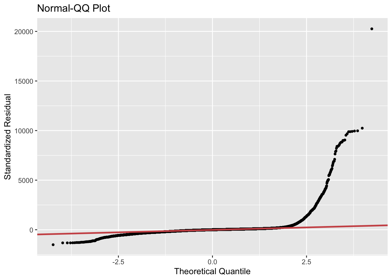We can see on the qqplot that our model has problems with the extreme values, mainly the very expensive properties. This could be expected knowing the “little” informations we had about the Airbnb listing.

3.2 Determine the value of a good by the price predicted and the criminality

In line with the methodology, we explained in the introduction, we will try to find a score multiplying the price predicted by our previous model and multiply it by a score.

In order to make our final prediction, we decided to use two different approaches:
* Using the criminality per 100’000 inhabitants
* Using the ciminality score defined in the Exploratory Data Analysis of the criminality

3.2.1 Using the criminality per 100’000 inhabitants

In this part, we are going to try to find the best model to predict the price of an Airbnb based on the prediction found with the previous equation (pred_price) and a combination of the differents types of criminality (using the crime per 100’000 inhabitants).

Firstly, we decided to use a model that multiply the predicted price from the previous model and multiply it by a score. This score is created by doing a linear combination of the different type of crimes per 100’000 inhabitants. This is the equation:

\(Price = \beta_1* pred\_price * (\beta_2 * violent\_crime + \beta_3*property\_crime + \\ \beta_4*crime\_murder\_or\_rape + \beta_5*robbery + \beta_6*burglary + \beta_7*vehicle\_crime)\)

Table 3.3: Accuracy of the multiplicative model without intercept
RMSE	MAE	MASE
356.642	115.097	0.755

## [1] "We have a r squared of 0.44"

Even though it is less intuitive, we decided to try an additive model where we add the previous mentionned score instead of multiplying by it. This is the equation:

\(Price = \beta_1* pred\_price + \beta_2 * violent\_crime + \beta_3*property\_crime + \\ \beta_4*crime\_murder\_or\_rape + \beta_5*robbery + \beta_6*burglary + \beta_7*vehicle\_crime\)

Table 3.4: Accuracy of the additive model with intercept
RMSE	MAE	MASE
364.765	124.404	0.816

## [1] "We have a r squared of 0.415"

Unsurprisingly, we notice that this model is yielding worse result than the first one we tested. Indeed we note that the \(R^2\) is smaller and that the MAE is bigger.

In conclusion, we found that the mutliplicative model has a better accuracy and \(R^2\).

3.2.2 Using the score created in the Exploratory Data Analysis

The second approach we wanted to try is one where the numeric value of the crimes per 100’000 inhabitants is replaced by the scores created in the crime Exploratory Data Analysis (based on the quantile of the crimes per 100’000 inhabitants). In line with our previous finding, We applied the same procedure.

We started with a multiplicative model with the following equation:

\(Price = \beta_1* pred\_price * (\beta_2 * score\_violent\_crime +\beta_3 * score\_property\_crime+ \\ \beta_4 * score\_crime\_murder\_or\_rape + \beta_5 * score\_robbery + \beta_6 * score\_burglary + \\ \beta_7 * score\_vehicle\_crime)\)

Table 3.5: Accuracy of the multiplicative model without intercept and score
RMSE	MAE	MASE
337.908	106.746	0.7

## [1] "We have a r squared of 0.498"

In line with the previous part, we tried an additive model following this equation:

\(Price = \beta_1* pred\_price + \beta_2 * score\_violent\_crime +\beta_3 * score\_property\_crime + \\ \beta_4 * score\_crime\_murder\_or\_rape + \beta_5 * score\_robbery + \beta_6 * score\_burglary + \\ \beta_7 * score\_vehicle\_crime\)

Table 3.6: Accuracy of the additive model with intercept
RMSE	MAE	MASE
360.86	126.505	0.83

## [1] "We have a r squared of 0.427"

The result from this section confirms our previous finding that a multiplicative model is more accurate and explain better the variance.

3.2.3 Comparing the best models

We decided to compare the best models from each subsection.

This is the result for the model using the criminality per 100’000 inhabitants:

Table 3.7: Accuracy of the multiplicative model without intercept and criminality per 100’000 inhabitants
RMSE	MAE	MASE
356.642	115.097	0.755

## [1] "We have a r squared of 0.44"

And this is the result for the model using the score:

Table 3.8: Accuracy of the multiplicative model without intercept and score
RMSE	MAE	MASE
337.908	106.746	0.7

## [1] "We have a r squared of 0.498"

Comparing them we found, we note that the model using the scores not only improve our explained variance \((R^2)\), but also increase significantly our accuracy by lowering the MAE by 8% to 106. Looking back at the accuracy we found in the model predicting the price from the characteristics, we have improved the accuracy by reducing the MAE by roughly 15%. Moreover, we increased the explained variance from 30% to nearly 50%!

3.3 Assessing the best model

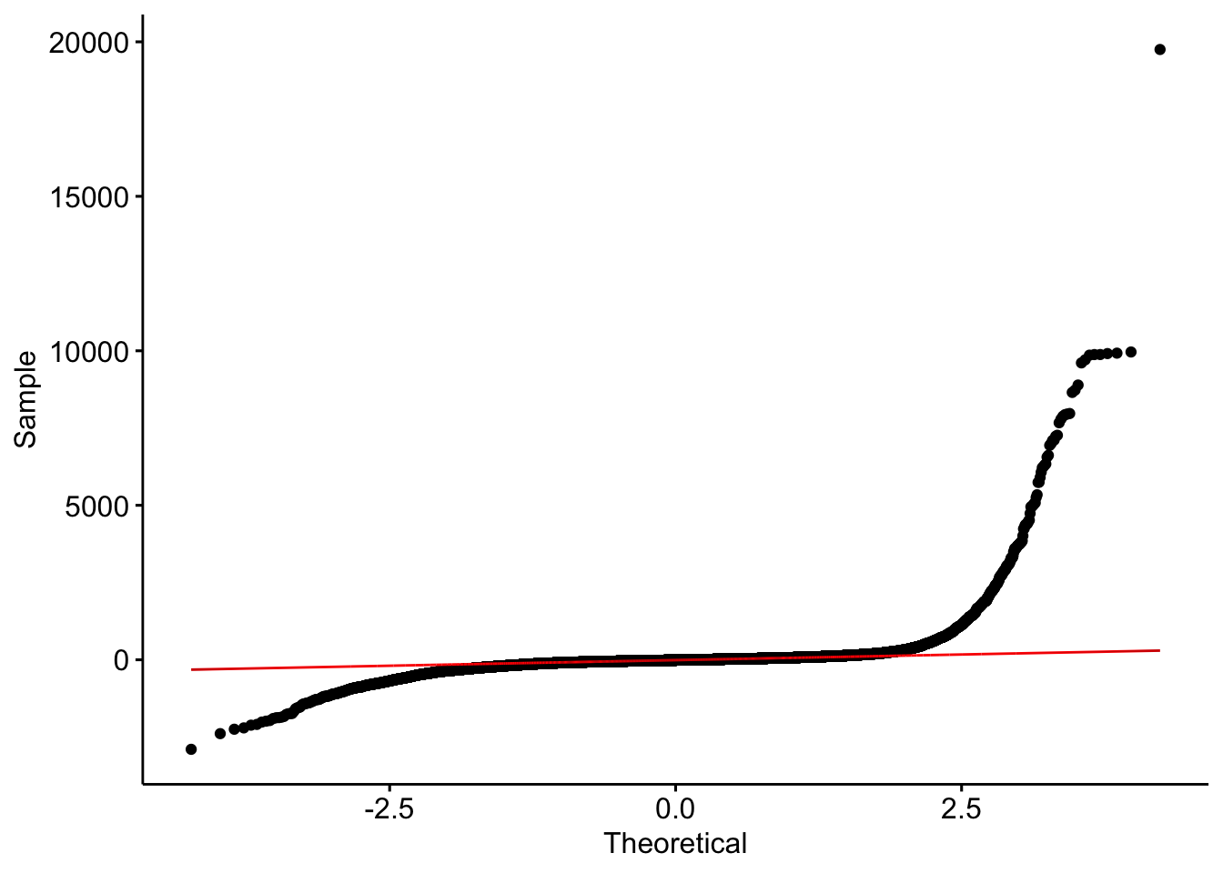
Following the result of our models, we decided to use the multiplicative model with the scores and no intercept.

Looking at the qqplot, we note that the still have the same global shape. We can conclude that the crimes are not sufficient to explain the very expensive listings. Unfortunately, we notice that the we decrease our precision for the really inexpensive places.

Looking at the distribution of the residuals, we notice that the errors are centered around 0. It is a sign of a good model as most of the listings price fall in a close interval of our model. This could be explained by the relatively low amount of information we have on the goods. We would need more precision regarding its type, condition, age, history,… Then, it could be argued that the criminality is not perfectly reflecting the value of a neighbourhood. Indeed, having a house next to the beach is impacted in the same way as a house located at the opposite side of the neighbourhood.