B Appendix B - R Code to read data, generate subgroups and analyze data
B.1 Libraries
B.2 Theory of change graph
B.3 Read and convert data
population <- as_tibble(read.csv("20190301CSTpopulation.csv"))
seen_Buddini <- as_tibble(read.csv("20190301CSTBuddini.csv"))
refugeeasylum <- as_tibble(read.csv("20190301CSTRefugeeAsylum.csv"))
# Calculate age
#
# By default, calculates the typical "age in years", with a
# \code{floor} applied so that you are, e.g., 5 years old from
# 5th birthday through the day before your 6th birthday. Set
# \code{floor = FALSE} to return decimal ages, and change \code{units}
# for units other than years.
# @param dob date-of-birth, the day to start calculating age.
# @param age.day the date on which age is to be calculated.
# @param units unit to measure age in. Defaults to \code{"years"}. Passed to \link{\code{duration}}.
# @param floor boolean for whether or not to floor the result. Defaults to \code{TRUE}.
# @return Age in \code{units}. Will be an integer if \code{floor = TRUE}.
# @examples
# my.dob <- as.Date('1983-10-20')
# age(my.dob)
# age(my.dob, units = "minutes")
# age(my.dob, floor = FALSE)
# code by 'Gregor'
# https://stackoverflow.com/questions/27096485/change-a-column-from-birth-date-to-age-in-r
# requires library 'lubridate'
age <- function(dob, age.day = today(), units = "years", floor = TRUE) {
calc.age = interval(dob, age.day) / duration(num = 1, units = units)
if (floor) return(as.integer(floor(calc.age)))
return(calc.age)
}
population <- population %>%
# add columns for whether they have seen the doctor who is making the telephone calls
# or are of known refugee or asylum seeker background
# (?proxy for low English language literacy)
mutate(SeenBuddini = INTERNALID %in% seen_Buddini$INTERNALID) %>%
mutate(RefugeeOrAsylum = INTERNALID %in% refugeeasylum$INTERNALID) %>%
mutate(Subgroup = case_when(
RefugeeOrAsylum & SeenBuddini ~ "Refugee+Buddini",
SeenBuddini ~ "Buddini",
RefugeeOrAsylum ~ "Refugee",
TRUE ~ "Standard"
)) %>%
mutate(Subgroup = as.factor(Subgroup)) %>%
mutate(DOB = dmy(DOB)) %>% # change into standard R date
mutate(Age = age(DOB, age.day = as.Date("2019/03/01"))) %>%
# note that age is on 1st March 2019
mutate(AgeGroup5 = as.factor((Age %/% 5)*5)) # 5-year age groups, labelled with minimum age
population %>%
dplyr::select("DOB", "Age", "SeenBuddini", "RefugeeOrAsylum",
"Subgroup", "AgeGroup5") %>%
summary()
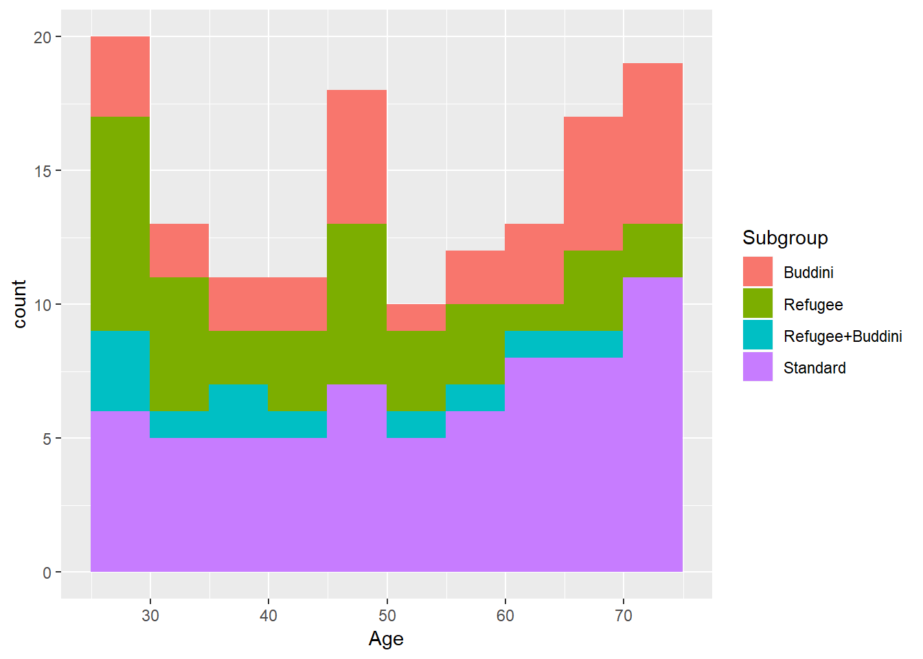
ggplot(population, aes(x = Age, fill=Subgroup)) +
geom_histogram(binwidth = 5, boundary = 25)B.4 Power calculation details
Previous proportion of under-screened patients who were screened in the three months after March 2018 was 5.2%. With a populaton of 290 patients, split between two groups, power of 0.8 and significance level of 0.05, the
power_3month <- power.prop.test(n = nrow(population)/2,
                                p1 = 0.05185,
                                # the measured proportion with recorded cervical screen
                                # under 'control' conditions
                                power=0.8, sig.level=0.05,
                                alternative = "two.sided")

power_3month

paste("Minimum detectable effect : ", round(power_3month$p2 - power_3month$p1, 4))
This is similar to estimated minimum detectable effect size using the equation:
\(EffectSize = (t_{1-\kappa}+t_\alpha)*\sqrt{\frac{1}{P(1-P)}}*\sqrt{\frac{\sigma^2}{N}}\)
where \(t_{1-\kappa}\) is the power, \(t_\alpha\) is the significance level, \(P\) is the proportion in treatment, \(\sigma^2\) is the variance and \(N\) is the sample size.
p1 <- 0.05185      # our previously observed proportion of women
# who had cervical screening (CST) over three months
p2 <- 0.1507374    # our 'guess' of what the 'treatment' group who had CST over
# three months. this guess was actually informed by
# above power calculation, however!
p_avg <- (p1+p2)/2 # the average proportion of women who might
# have cervical screening at the end of the study
# variance of binomial is p(1-p)

abs(qnorm(0.8)+qnorm(0.975))*sqrt(1/((0.5)*(1-0.5)))*sqrt((p_avg)*(1-p_avg)/290)
## [1] 0.09927387Previous proportion of under-screened patients who were screened in the six months after March 2018 was 8.9%. With a populaton of 290 patients, split between two groups, power of 0.8 and significance level of 0.05:
power_6month <- power.prop.test(n = nrow(population)/2,
                                p1 = 0.08889,
                                # the measured proportion with recorded cervical screen
                                # under 'control' conditions
                                power=0.8, sig.level=0.05,
                                alternative = "two.sided")

power_6month
##
## Two-sample comparison of proportions power calculation
##
## n = 145
## p1 = 0.08889
## p2 = 0.2049093
## sig.level = 0.05
## power = 0.8
## alternative = two.sided
##
## NOTE: n is number in *each* group## [1] "Minimum detectable effect : 0.116019322103659"B.5 Randomized allocation
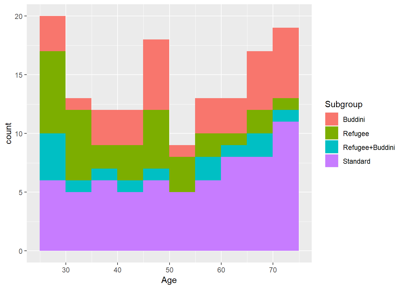
ggplot(treatment, aes(x = Age, fill=Subgroup)) +
  geom_histogram(binwidth = 5, boundary = 24.95)
ggplot(control, aes(x = Age, fill=Subgroup)) +
  geom_histogram(binwidth = 5, boundary = 24.95)
B.5.1 Phase 1 group characteristics
B.6 Survey team allocation
set.seed(1603104944)

treatment1 <- NULL
treatment2 <- NULL

for (i in levels(treatment$AgeGroup5)) {
  coinflip <- runif(1)>.5
  for (j in levels(treatment$Subgroup)) {
    subsection <- treatment[treatment$AgeGroup5 == i & treatment$Subgroup == j,]
    subsection$rank <- runif(nrow(subsection))
    if ((nrow(subsection) %% 2) == 1)
    {coinflip <- 1 - coinflip} # toggle from favouring one group or another
    new_treatment1 <- top_n(subsection, as.integer(nrow(subsection)/2 + coinflip*.5), rank)
    new_treatment2 <- anti_join(subsection, new_treatment1, by = "INTERNALID")
    treatment1 <- rbind(treatment1, new_treatment1)
    treatment2 <- rbind(treatment2, new_treatment2)
  }
}

control1 <- NULL
control2 <- NULL

for (i in levels(control$AgeGroup5)) {
  coinflip <- runif(1)>.5
  for (j in levels(control$Subgroup)) {
    subsection <- control[control$AgeGroup5 == i & control$Subgroup == j,]
    subsection$rank <- runif(nrow(subsection))
    if ((nrow(subsection) %% 2) == 1)
    {coinflip <- 1 - coinflip} # toggle from favouring one group or another
    new_control1 <- top_n(subsection, as.integer(nrow(subsection)/2 + coinflip*.5), rank)
    new_control2 <- anti_join(subsection, new_control1, by = "INTERNALID")
    control1 <- rbind(control1, new_control1)
    control2 <- rbind(control2, new_control2)
  }
}
Phase 1, group 1
Phase 1, group 2
Phase 2, group 1
Phase 2, group 2
B.7 Export sub-groups to Excel file for surveyor use.
Re-attach patient names and demographic details to sub-groups, and export to Excel file (Phase 1 = Treat, Phase 2 = Control) for use by surveyors.
# set {r eval = FALSE when 'knitting' to form a HTML file}
# as identifying data should not be in a public space!

patient_details <- read.csv("20190301CSTpopulation_details.csv")
# file with patient details
patient_details <- patient_details %>%
  select(c("INTERNALID", "SURNAME", "FIRSTNAME", "MIDDLENAME", "PREFERREDNAME", "TITLE", "DOB", "AGE", "RECORDNO"))
# select columns required for export

treatment1_details <- treatment1 %>%
  select(c("INTERNALID", "AgeGroup5")) %>%
  # will store AgeGroup5 groups in separate sheets
  left_join(patient_details, by = "INTERNALID")

treatment2_details <- treatment2 %>%
  select(c("INTERNALID", "AgeGroup5")) %>%
  # will store AgeGroup5 groups treatment in separate sheets
  left_join(patient_details, by = "INTERNALID")

control1_details <- control1 %>%
  select(c("INTERNALID", "AgeGroup5")) %>%
  # will store AgeGroup5 groups in separate sheets
  left_join(patient_details, by = "INTERNALID")

control2_details <- control2 %>%
  select(c("INTERNALID", "AgeGroup5")) %>%
  # will store AgeGroup5 groups in separate sheets
  left_join(patient_details, by = "INTERNALID")

wb_treat <- createWorkbook() # create blank workbook

for (i in levels(treatment1_details$AgeGroup5)) {
  subsection1 <- treatment1_details[treatment1_details$AgeGroup5 == i,]
  sheetname1 <- paste("Phase 1 Group 1 - ", i)
  addWorksheet(wb_treat, sheetname1)
  writeData(wb_treat, sheetname1, subsection1)
  subsection2 <- treatment2_details[treatment2_details$AgeGroup5 == i,]
  sheetname2 <- paste("Phase 1 Group 2 - ", i)
  addWorksheet(wb_treat, sheetname2)
  writeData(wb_treat, sheetname2, subsection2)
}

saveWorkbook(wb_treat, file = "20190301CSTPhase1Groups.xlsx", overwrite = TRUE)

wb_control <- createWorkbook() # create blank workbook

for (i in levels(control1_details$AgeGroup5)) {
  subsection1 <- control1_details[control1_details$AgeGroup5 == i,]
  sheetname1 <- paste("Phase 2 Group 1 - ", i)
  addWorksheet(wb_control, sheetname1)
  writeData(wb_control, sheetname1, subsection1)
  subsection2 <- control2_details[control2_details$AgeGroup5 == i,]
  sheetname2 <- paste("Phase 2 Group 2 - ", i)
  addWorksheet(wb_control, sheetname2)
  writeData(wb_control, sheetname2, subsection2)
}

saveWorkbook(wb_control, file = "20190301CSTPhase2Groups.xlsx", overwrite = TRUE)
B.8 Results
# reads results and processes

xl1_name <- '20190401CSTPhase1Groups_results_20191114.xlsx' # results held in these XLSX spreadsheets
xl2_name <- '20190401CSTPhase2Groups_results_20191114.xlsx'

sheet_names <- getSheetNames(xl1_name) # not actually used

# the phase 1 groups who have been contacted as of 14th November 2019
id1_1_25 <- read.xlsx(xl1_name, sheet = "Phase 1 Group 1 -  25") %>%
  pull(INTERNALID)
id1_2_25 <- read.xlsx(xl1_name, sheet = "Phase 1 Group 2 -  25") %>%
  pull(INTERNALID)
id1_2_30 <- read.xlsx(xl1_name, sheet = "Phase 1 Group 2 -  30") %>%
  pull(INTERNALID)
id1_2_35 <- read.xlsx(xl1_name, sheet = "Phase 1 Group 2 -  35") %>%
  pull(INTERNALID)

id1b <- c(id1_2_25, id1_2_30, id1_2_35) # 'phase1' group contact by BE
id1 <- c(id1_1_25, id1b) # total phase 1 group contacted

# the comparison phase 2 groups (aged 25-40), not contacted by telephone
id2_1_25 <- read.xlsx(xl2_name, sheet = "Phase 2 Group 1 -  25") %>%
  pull(INTERNALID)
id2_1_30 <- read.xlsx(xl2_name, sheet = "Phase 2 Group 1 -  30") %>%
  pull(INTERNALID)
id2_1_35 <- read.xlsx(xl2_name, sheet = "Phase 2 Group 1 -  35") %>%
  pull(INTERNALID)
id2_2_25 <- read.xlsx(xl2_name, sheet = "Phase 2 Group 2 -  25") %>%
  pull(INTERNALID)
id2_2_30 <- read.xlsx(xl2_name, sheet = "Phase 2 Group 2 -  30") %>%
  pull(INTERNALID)
id2_2_35 <- read.xlsx(xl2_name, sheet = "Phase 2 Group 2 -  35") %>%
  pull(INTERNALID)

# equivalent phase 2 group
id2 <- c(id2_1_25, id2_2_25, id2_1_30, id2_2_30, id2_1_35, id2_2_35)

# all the IDs in the phase 1 (contacted) and phase 2 (not contacted)
id <- c(id1, id2)
df <- data.frame(InternalID = id)

df <- df %>%
  mutate(Phase = InternalID %in% id1) # Phase is 'TRUE' if Phase 1

# as of 14th November 2019, the CSV list of those with no CST
# in the past two years (2 years ago, the CST was 'Pap', which
# is due in two years)
noCST1 <- read.csv("TelephoneCST_Phase1_NoCST.csv")
noCST2 <- read.csv("TelephoneCST_Phase2_NoCST.csv")

noCST1_id <- noCST1 %>% pull(INTERNALID) # just get the IDs
noCST2_id <- noCST2 %>% pull(INTERNALID)
noCST_ID <- c(noCST1_id, noCST2_id) # combine the IDs

df <- df %>%
  mutate(CST = !(InternalID %in% noCST_ID))
# CST is TRUE if 'not' in the 'no CST' list

seenby_Buddini <- read.csv("20190401CSTBuddini.csv")
seenby_Buddini_id <- seenby_Buddini %>% pull(INTERNALID)

df <- df %>%
  mutate(Group2 = InternalID %in% id1b,
         Buddini = InternalID %in% seenby_Buddini_id)
# currently 'Group2' are those contacted by BE
# currently 'Buddini' are those who have previously been seen by BE

refugee_asylum <- read.csv("20190401CSTRefugeeAsylum.csv")
refugee_asylum_id <- refugee_asylum %>% pull(INTERNALID)

df <- df %>%
  mutate(refugee = InternalID %in% refugee_asylum_id)
# those listed as asylum or refugee status

df_tab <- data.frame(CSTfalse = numeric(), CSTtrue = numeric())

a <- by(df$CST, df$CST, length) # both refugee and non-refugee groups, in both phases
df_tab <- rbind(df_tab, n = data.frame(CSTfalse = a[1], CSTtrue = a[2]))
a <- by(subset(df$CST, df$Phase), subset(df$CST, df$Phase), length) # phase 1
df_tab <- rbind(df_tab, Phase1 = data.frame(CSTfalse = a[1], CSTtrue = a[2]))
a <- by(subset(df$CST, !df$Phase), subset(df$CST, !df$Phase), length) #phase 2
df_tab <- rbind(df_tab, Phase2 = data.frame(CSTfalse = a[1], CSTtrue = a[2]))

a <- by(subset(df$CST, df$refugee), subset(df$CST, df$refugee), length) # refugee subset
df_tab <- rbind(df_tab, `n ` = data.frame(CSTfalse = a[1], CSTtrue = a[2]))
# extra space avoids duplicate rowname problem
a <- by(subset(df$CST, df$refugee & df$Phase), subset(df$CST, df$refugee & df$Phase), length)
df_tab <- rbind(df_tab, `Phase1 ` = data.frame(CSTfalse = a[1], CSTtrue = a[2]))
a <- by(subset(df$CST, df$refugee & !df$Phase), subset(df$CST, df$refugee & !df$Phase), length)
df_tab <- rbind(df_tab, `Phase2 `= data.frame(CSTfalse = a[1], CSTtrue = a[2]))

a <- by(subset(df$CST, !df$refugee), subset(df$CST, !df$refugee), length) # non-refugee subset
df_tab <- rbind(df_tab, `n  ` = data.frame(CSTfalse = a[1], CSTtrue = a[2]))
a <- by(subset(df$CST, !df$refugee & df$Phase), subset(df$CST, !df$refugee & df$Phase), length)
df_tab <- rbind(df_tab, `Phase1  ` = data.frame(CSTfalse = a[1], CSTtrue = a[2]))
a <- by(subset(df$CST, !df$refugee & !df$Phase), subset(df$CST, !df$refugee & !df$Phase), length)
df_tab <- rbind(df_tab, `Phase2  ` = data.frame(CSTfalse = a[1], CSTtrue = a[2]))

df_tab$CSTfalseProp <- df_tab$CSTfalse/(df_tab$CSTfalse+df_tab$CSTtrue)
df_tab$CSTtrueProp <- df_tab$CSTtrue/(df_tab$CSTfalse+df_tab$CSTtrue)

df_tab <- df_tab[, c("CSTfalse", "CSTfalseProp", "CSTtrue", "CSTtrueProp")]
df_tab %>%
  mutate(Group = row.names(.),
         CSTfalseProp = color_tile("#DeF7E9", "#71CA97")(percent(CSTfalseProp, 1)),
         CSTtrueProp= color_tile("#DeF7E9", "#71CA97")(percent(CSTtrueProp, 1))) %>%
  dplyr::select(Group, everything()) %>%
  kable("html", escape = F,
        col.names = c(" ", "n", "%", "n", "%"),
        booktabs = TRUE,
        caption = 'Cervical screening recall results')  %>%
  kable_styling("striped", full_width = F) %>%
  column_spec(1, width = "10em") %>%
  row_spec(0, align = "c") %>%
  add_header_above(c(" " = 1, "CST overdue" = 2, "CST done" = 2)) %>%
  pack_rows("All", 1, 3) %>%
  pack_rows("Refugee", 4, 6) %>%
  pack_rows("Other", 7, 9)

interaction.plot(df$Phase, df$refugee, df$CST,
                 trace.label = "Refugee",
                 xlab = "Telephone recall",
                 ylab = "Cervical Screening up-to-date (proportion)")
model1 <- glm(CST ~ refugee * Phase, family = binomial(link = "logit"), data = df)
model2 <- stepAIC(model1, trace = FALSE)
# the 'best' model, combining explanatory power and simplicity, accord ing to the
# stepwise Akaiki Information Criterion (AIC) selection
huxreg("Refugee model" = model1, "Simple model" = model2) %>%
  huxtable::set_caption("Refugee/Asylum-seeker status as a predictor of response to telephone-based recall") %>%
  huxtable::set_label("tab:aic")