Section 2 Week 1 - November 18, 2022
2.1 R Layout
This was our first meeting. The group was introduced to the R interface, including the various panes (i.e., sections of RStudio) and what they are used for.
The bottom-left (given you are using the default lay out) is the console, where code runs. You can type code directly into the console. For example, you can run some basic maths (type or copy and paste the following into your console):
5 + 6# ^ indicates exponent
25^3 # sqrt() is square root
sqrt(16)The top-left is your current script. If you don’t have one open - typically, you will see a name such as ‘Untitled1’ - you can open one by clicking File -> New File -> R Script or CTRL + SHIFT + N (Windows)/ CMD+SHIFT+N (Mac). Scripts are a great way to organize and save your code. We will use scripts throughout our meetings.
The bottom-right has a few different functions. It’s used top view files, such as those in your working directory (where R will automatically try to load or save files), view figures/plots, and get help (e.g., view documentation).
The top-right pane is the environment and displays all current objects being used by R. For example, it could display data sets, values, functions, etc. You can create objects by using the following structure object name <- what the object is. Note, the keyboard shortcut for ‘<-’ is ALT + - (Windows)/FUNCTION + - (Mac). For example, if I wanted to create an object called hello that was just the number 5, I could run:
hello <- 5Or I could make a object called ‘scores’ that is a list of numbers, ‘5, 2, 4, 2, 1’:
scores <- c(5, 2, 4, 2, 1)Note that c() means concatenate (things together in a series) and that you must separate things by a comma.
2.2 Variable Types
Much like SPSS, there are several variable types. We will primarily be concerned with: numeric, factor, and character. Numeric is easy enough to understand. Factors are ‘words’ or ‘strings’ that get stored as a number that is a level. For example, ‘color’ might have the levels: ‘red’, ‘blue’, and ‘green’. Storing as a factor allows for easy comparison of colors; every who selects ‘red’ will be group at that level of a factors. Characters do not work this way, so it will be important to ensure your factors are indeed factors.
You can store factors/characters as objects as well. Let’s create an object called ‘Tyler’ that contains my last name, favorite number, and favorite color. Note: strings must be contained in ” ” (object names do not follow this rule).
Tyler <- c("Pritchard", 23, "Blue")2.3 Installing Packages
We discussed how R is like an iPhone. While it comes with awesome things you will use a lot, like Camera and Photos, you may want to download some extra apps. Apps are like R packages/libraries. One package we will use a lot are those from the tidyverse. You can download this package by using the bottom-right pane. Packages -> Install -> tidyverse. Or, you could run a script (note: you must put the package name in quotation marks ’ ’ or ” “):
install.packages('tidyverse')Not only must you download packages, you must run them if you want to use them. Imagine trying to take a photo on your phone, you can’t just hold it up and say ‘take photo’, you must first click the ‘Camera’ app. Loading a package in R is like clicking an app you want to use. Every time you close R, all you packages (‘apps’) will be exited; so, you must re-run the package when you open R again. You run a package using library(), with the package in brackets. So:
library(tidyverse)2.4 Functions
Functions can do so many things. We will not focus on creating functions right now, only using existing ones. You will use them all the time when using R. You can call on functions by typing their name. They typically are followed by brackets that have arguments in them. Arguments are like choices that you must specify for the function to run. Some arguments have default values, which means that you do not need to change or specify anything with them unless needed.
Functions can calculate statistics, create figures, generate data, send a Tweet, download data from Google, etc. Also, as mentioned, you can create functions to do whatever you like.
Let’s use a simple function to calculate the mean of the ‘scores’, the object we made above. R comes with many built in functions, including mean(). As you type a function, the arguments may display on your screen. Otherwise, you can run the function with a ‘?’ it to have the help documentation pop up in the bottom-right pane.
?mean()For mean, the only thing we need to specify if the object on which we want to calculate the mean. So:
mean(scores)## [1] 2.8The mean of ‘scores’ is 2.8.
Another common function you may use is sd(), which calculates the standard deviation of a set of values.
sd(scores)## [1] 1.6431682.5 Using Data
Most of the time, you will likely not be using a vector (which is what our object ‘scores’ is). You will be using a set of data. In R, we can call this a data.frame (tibbles also exist, but we will primarily use data frames). R comes with some built in data frames, so let’s store one in the environment.
df <- mtcarsand it looks something like this:
| mpg | cyl | disp | hp | drat | wt | qsec | vs | am | gear | carb | |
|---|---|---|---|---|---|---|---|---|---|---|---|
| Mazda RX4 | 21.0 | 6 | 160.0 | 110 | 3.90 | 2.620 | 16.46 | 0 | 1 | 4 | 4 |
| Mazda RX4 Wag | 21.0 | 6 | 160.0 | 110 | 3.90 | 2.875 | 17.02 | 0 | 1 | 4 | 4 |
| Datsun 710 | 22.8 | 4 | 108.0 | 93 | 3.85 | 2.320 | 18.61 | 1 | 1 | 4 | 1 |
| Hornet 4 Drive | 21.4 | 6 | 258.0 | 110 | 3.08 | 3.215 | 19.44 | 1 | 0 | 3 | 1 |
| Hornet Sportabout | 18.7 | 8 | 360.0 | 175 | 3.15 | 3.440 | 17.02 | 0 | 0 | 3 | 2 |
| Valiant | 18.1 | 6 | 225.0 | 105 | 2.76 | 3.460 | 20.22 | 1 | 0 | 3 | 1 |
| Duster 360 | 14.3 | 8 | 360.0 | 245 | 3.21 | 3.570 | 15.84 | 0 | 0 | 3 | 4 |
| Merc 240D | 24.4 | 4 | 146.7 | 62 | 3.69 | 3.190 | 20.00 | 1 | 0 | 4 | 2 |
| Merc 230 | 22.8 | 4 | 140.8 | 95 | 3.92 | 3.150 | 22.90 | 1 | 0 | 4 | 2 |
| Merc 280 | 19.2 | 6 | 167.6 | 123 | 3.92 | 3.440 | 18.30 | 1 | 0 | 4 | 4 |
| Merc 280C | 17.8 | 6 | 167.6 | 123 | 3.92 | 3.440 | 18.90 | 1 | 0 | 4 | 4 |
| Merc 450SE | 16.4 | 8 | 275.8 | 180 | 3.07 | 4.070 | 17.40 | 0 | 0 | 3 | 3 |
| Merc 450SL | 17.3 | 8 | 275.8 | 180 | 3.07 | 3.730 | 17.60 | 0 | 0 | 3 | 3 |
| Merc 450SLC | 15.2 | 8 | 275.8 | 180 | 3.07 | 3.780 | 18.00 | 0 | 0 | 3 | 3 |
| Cadillac Fleetwood | 10.4 | 8 | 472.0 | 205 | 2.93 | 5.250 | 17.98 | 0 | 0 | 3 | 4 |
| Lincoln Continental | 10.4 | 8 | 460.0 | 215 | 3.00 | 5.424 | 17.82 | 0 | 0 | 3 | 4 |
| Chrysler Imperial | 14.7 | 8 | 440.0 | 230 | 3.23 | 5.345 | 17.42 | 0 | 0 | 3 | 4 |
| Fiat 128 | 32.4 | 4 | 78.7 | 66 | 4.08 | 2.200 | 19.47 | 1 | 1 | 4 | 1 |
| Honda Civic | 30.4 | 4 | 75.7 | 52 | 4.93 | 1.615 | 18.52 | 1 | 1 | 4 | 2 |
| Toyota Corolla | 33.9 | 4 | 71.1 | 65 | 4.22 | 1.835 | 19.90 | 1 | 1 | 4 | 1 |
| Toyota Corona | 21.5 | 4 | 120.1 | 97 | 3.70 | 2.465 | 20.01 | 1 | 0 | 3 | 1 |
| Dodge Challenger | 15.5 | 8 | 318.0 | 150 | 2.76 | 3.520 | 16.87 | 0 | 0 | 3 | 2 |
| AMC Javelin | 15.2 | 8 | 304.0 | 150 | 3.15 | 3.435 | 17.30 | 0 | 0 | 3 | 2 |
| Camaro Z28 | 13.3 | 8 | 350.0 | 245 | 3.73 | 3.840 | 15.41 | 0 | 0 | 3 | 4 |
| Pontiac Firebird | 19.2 | 8 | 400.0 | 175 | 3.08 | 3.845 | 17.05 | 0 | 0 | 3 | 2 |
| Fiat X1-9 | 27.3 | 4 | 79.0 | 66 | 4.08 | 1.935 | 18.90 | 1 | 1 | 4 | 1 |
| Porsche 914-2 | 26.0 | 4 | 120.3 | 91 | 4.43 | 2.140 | 16.70 | 0 | 1 | 5 | 2 |
| Lotus Europa | 30.4 | 4 | 95.1 | 113 | 3.77 | 1.513 | 16.90 | 1 | 1 | 5 | 2 |
| Ford Pantera L | 15.8 | 8 | 351.0 | 264 | 4.22 | 3.170 | 14.50 | 0 | 1 | 5 | 4 |
| Ferrari Dino | 19.7 | 6 | 145.0 | 175 | 3.62 | 2.770 | 15.50 | 0 | 1 | 5 | 6 |
| Maserati Bora | 15.0 | 8 | 301.0 | 335 | 3.54 | 3.570 | 14.60 | 0 | 1 | 5 | 8 |
| Volvo 142E | 21.4 | 4 | 121.0 | 109 | 4.11 | 2.780 | 18.60 | 1 | 1 | 4 | 2 |
We can quickly look at the data structure using the str() function.
str(df)## 'data.frame': 32 obs. of 11 variables:
## $ mpg : num 21 21 22.8 21.4 18.7 18.1 14.3 24.4 22.8 19.2 ...
## $ cyl : num 6 6 4 6 8 6 8 4 4 6 ...
## $ disp: num 160 160 108 258 360 ...
## $ hp : num 110 110 93 110 175 105 245 62 95 123 ...
## $ drat: num 3.9 3.9 3.85 3.08 3.15 2.76 3.21 3.69 3.92 3.92 ...
## $ wt : num 2.62 2.88 2.32 3.21 3.44 ...
## $ qsec: num 16.5 17 18.6 19.4 17 ...
## $ vs : num 0 0 1 1 0 1 0 1 1 1 ...
## $ am : num 1 1 1 0 0 0 0 0 0 0 ...
## $ gear: num 4 4 4 3 3 3 3 4 4 4 ...
## $ carb: num 4 4 1 1 2 1 4 2 2 4 ...Here, you can see the names of the variables, their types, and the first few values.
Remember the mean() function? It needed a set of data to calculate mean on. Let’s try to calculate the mean of a variable in the data set we just put in the environment.
To call a specific variable in a data.frame, we must name the data frame, put ‘$’, and then list the variable. Let’s calculate the mean of the miles per gallon variable, ‘mpg’.
mean(df$mpg)## [1] 20.090622.6 Quick Plots
You can quickly plot with the plot() function. It will take the variables you put in the function and try to make the best type of figure. Let’s plot two variables from our data set: mpg (miles per gallon) and hp (horsepower).
plot(df$mpg, df$hp)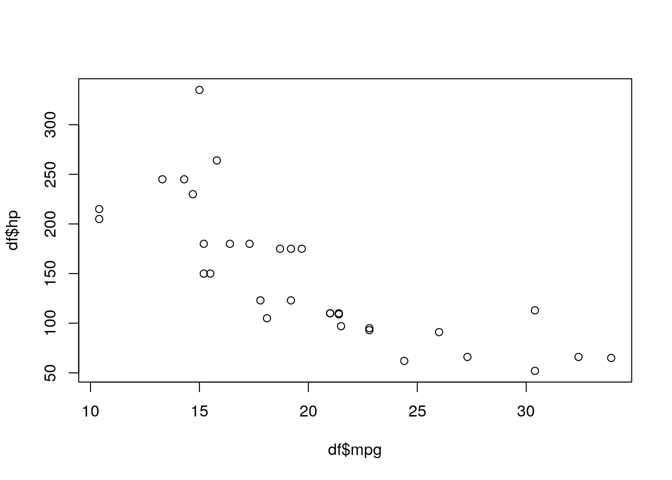
2.7 Quick Correlation NHST
R also has a quick function to do a NHST for a correlation: cor.test(). Let’s run a correlation on the variables from above. The help documentation (remember ?cot.test()) indicates that the only arguments we need to specify are x and y. Let x be mpg and y be hp:
cor.test(df$mpg, df$hp)##
## Pearson's product-moment correlation
##
## data: df$mpg and df$hp
## t = -6.7424, df = 30, p-value = 1.788e-07
## alternative hypothesis: true correlation is not equal to 0
## 95 percent confidence interval:
## -0.8852686 -0.5860994
## sample estimates:
## cor
## -0.7761684The results suggest that these data are unlikely given a true null.
That’s all we covered this week!
2.8 Practice questions
Install the ‘dplyr’ package.
Load the
starwarsdata set into the environment. Give it the name ‘sw’.Calculate the mean of height of the Star Wars characters.
- Hint: the mean() function defaults an argument
na.rmto FALSE. This will keep values of NA. You will have to remove NAs. Change the argument to remove NAs.