Chapter 9 Positive Definite Matrices
9.1 Terminology
A \(n \times n\) symmetric matrix \(M\) is positive definite (PD) if and only if \(x'Mx > 0\), for all non-zero \(x \in \mathbb{R}^n\). For example, take the \(3 \times 3\) identity matrix, and a column vector of non-zero real numbers \([a,b,c]\):
\[ \begin{aligned} \begin{bmatrix} a & b & c \end{bmatrix} \begin{bmatrix} 1 & 0 & 0\\ 0 & 1 & 0 \\ 0 & 0 & 1 \end{bmatrix} \begin{bmatrix} a \\ b \\ c \end{bmatrix} \\ = \begin{bmatrix} a & b & c \end{bmatrix} \begin{bmatrix} a \\ b \\ c \end{bmatrix} \\ = a^2 + b^2 + c^2. \end{aligned} \]
Since by definition \(a^2, b^2,\) and \(c^2\) are all greater than zero (even if \(a,b,\) or \(c\) are negative), their sum is also positive.
A matrix is positive semi-definite (PSD) if and only if \(x'Mx \geq 0\) for all non-zero \(x \in \mathbb{R}^n\). Note that PSD differs from PD in that the transformation of the matrix is no longer strictly positive.
One known feature of matrices (that will be useful later in this chapter) is that if a matrix is symmetric and idempotent then it will be positive semi-definite. Take some non-zero vector \(x\), and a symmetric, idempotent matrix \(A\). By idempotency we know that \(x'Ax = x'AAx\). By symmetry we know that \(A' = A\), and therefore:
\[ \begin{aligned} x'Ax &= x'AAx \\ &= x'A'Ax \\ &= (Ax)'Ax \geq 0, \end{aligned} \]
and hence PSD.16
9.1.1 Positivity
Both PD and PSD are concerned with positivity. For scalar values like -2, 5, 89, positivity simply refers to their sign – and we can tell immediately whether the numbers are positive or not. Some functions are also (strictly) positive. Think about \(f(x) = x^2 + 1\). For all \(x \in \mathbb{R}\), \(f(x) \geq 1 > 0\). PD and PSD extend this notion of a positivity to matrices, which is useful when we consider multidimensional optimisation problems or the combination of matrices.
While for abstract matrices like the identity matrix it is easy to verify PD and PSD properties, for more complicated matrices we often require other more complicated methods. For example, we know that a symmetric matrix is PSD if and only if all its eigenvalues are non-negative. The eigenvalue \(\lambda\) is a scalar such that, for a matrix \(A\) and non-zero \(n\times 1\) vector \(v\), \(A\cdot v = \lambda \cdot v\). While I do not explore this further in this chapter, there are methods available for recovering these values from the preceding equation. Further discussion of the full properties of PD and PSD matrices can be found here as well as in print (e.g. Horn and Johnson 2013, chap. 7).
9.2 \(A-B\) is PSD iff \(B^{-1} - A^{-1}\) is PSD
Wooldridge’s list of 10 theorems does not actually include a general claim about the importance P(S)D matrices. Instead, he lists a very specific feature of two PD matrices. In plain English, this theorem states that, assuming \(A\) and \(B\) are both positive definite, \(A-B\) is positive semi-definite if and only if the inverse of \(B\) minus the inverse of \(A\) is positive semi-definite.
Before we prove this theorem, it’s worth noting a few points that are immediately intuitive from its statement. Note that the theorem moves from PD matrices to PSD matrices. This is because we are subtracting one matrix from another. While we know A and B are both PD, if they are both equal then \(x'(A-B)x\) will equal zero. For example, if \(A = B = I_2 = \big(\begin{smallmatrix} 1 & 0\\ 0 & 1 \end{smallmatrix}\big)\), then \(A-B = \big(\begin{smallmatrix} 0 & 0\\ 0 & 0 \end{smallmatrix}\big)\). Hence, \(x'(A-B)x = 0\) and therefore \(A-B\) is PSD, but not PD.
Also note that this theorem only applies to a certain class of matrices, namely those we know to be PD. This hints at the sort of applied relevance this theorem may have. For instance, we know that variance is a strictly positive quantity.
The actual applied relevance of this theorem is not particularly obvious, at least from the claim alone. In his post, Wooldridge notes that he repeatedly uses this fact ‘to show the asymptotic efficiency of various estimators.’ In his Introductory Economics textbook (2013), for instance, Wooldridge makes use of the properties of PSD matrices in proving that the Gauss-Markov (GM) assumptions ensure that OLS is the best, linear, unbiased estimator (BLUE). And, more generally, PD and PSD matrices are very helpful in optimisation problems (of relevance to machine learning too). Neither appear to be direct applications of this specific, bidirectional theorem. In the remainder of this chapter, therefore, I prove the theorem itself for completeness. I then broaden the discussion to explore how PSD properties are used in Wooldridge’s BLUE proof as well as discuss the more general role of PD matrices in optimisation problems.
9.2.1 Proof
The proof of Wooldridge’s actual claim is straightforward. In fact, given the symmetry of the proof, we only need to prove one direction (i.e. if \(A-B\) is PSD, then \(A^{-1} - B^{-1}\) is PSD.)
Let’s assume, therefore, that \(A - B\) is PSD. Hence:
\[ \begin{aligned} x'(A-B)x &\geq 0 \\ x'Ax - xBx &\geq 0 \\ x'Ax &\geq x'Bx \\ Ax &\geq Bx \\ A &\geq B. \end{aligned} \]
Next, we can invert our two matrices while maintaining the inequality:
\[ \begin{aligned} A^{-1}AB^{-1} &\geq A^{-1}BB^{-1} \\ IB^{-1} &\geq A^{-1}I \\ B^{-1} &\geq A^{-1}. \end{aligned} \]
Finally, we can just remultiply both sides of the inequality by our arbitrary non-zero vector:
\[ \begin{aligned} x'B^{-1} &\geq x'A^{-1} \\ x'B^{-1}x &\geq x'A^{-1}x \\ x'B^{-1}x - x'A^{-1}x &\geq 0 \\ x'(B^{-1} - A^{-1})x &\geq 0. \end{aligned} \]
Proving the opposite direction (if \(B^{-1} - A^{-1}\) is PSD then \(A-B\) is PSD) simply involves replacing A with \(B^{-1}\) an \(B\) with \(A^{-1}\) and vice versa throughout the proof, since \((A^{-1})^{-1} = A. \;\;\;\square\)
9.3 Applications
9.3.1 OLS as the best linear unbiased estimator (BLUE)
First, let’s introduce the four Gauss-Markov assumptions. I only state these briefly, in the interest of space, spending a little more time explaining the rank of a matrix. Collectively, these assumptions guarantee that the linear regression estimates \(\hat{\beta}\) are BLUE (the best linear unbiased estimator of \(\beta\)).
The true model is linear such that \(y = X\beta + u\), where \(y\) is a \(n \times 1\) vector, \(X\) is a \(n \times (k + 1)\) matrix, and \(u\) is an unobserved \(n \times 1\) vector.
The rank of \(X\) is \((k+1)\) (full-rank), i.e. that there are no linear dependencies among the variables in \(X\). To understand what the rank of matrix denotes, consider the following \(3\times 3\) matrix:
\[ M_1=\begin{bmatrix} 1 & 0 & 0 \\ 0 & 1 & 0 \\ 2 & 0 & 0 \end{bmatrix} \]
Note that the third row of \(M_1\) is just two times the first column. They are therefore entirely linearly dependent, and so not separable. The number of independent rows (the rank of the matrix) is therefore 2. One way to think about this geometrically, as in Chapter 3, is to plot each row as a vector. The third vector would completely overlap the first, and so in terms of direction we would not be able to discern between them. In terms of the span of these two columns, moreover, there is no point that one can get to using a combination of both that one could not get to by scaling either one of them.
A slightly more complicated rank-deficient (i.e. not full rank) matrix would be:
\[ M_2=\begin{bmatrix} 1 & 0 & 0 \\ 0 & 1 & 0 \\ 2 & 1 & 0 \end{bmatrix} \]
Here note that the third row is not scalar multiple of either other column. But, it is a linear combination of the other two. If rows 1, 2, and 3 are represented by \(a, b,\) and \(c\) respectively, then \(c = 2a + b\). Again, geometrically, there is no point that the third row vector can take us to which cannot be achieved using only the first two rows.
An example of a matrix with full-rank, i.e. no linear dependencies, would be:
\[ M_2=\begin{bmatrix} 1 & 0 & 0 \\ 0 & 1 & 0 \\ 2 & 0 & 1 \end{bmatrix} \]
It is easy to verify that \(M_1\) and \(M_2\) are rank-deficient, whereas \(M_3\) is of full-rank in R:
M1 <- matrix(c(1,0,2,0,1,0,0,0,0), ncol = 3)
M1_rank <- qr(M1)$rank

M2 <- matrix(c(1,0,2,0,1,1,0,0,0), ncol = 3)
M2_rank <- qr(M2)$rank

M3 <- matrix(c(1,0,2,0,1,0,0,0,1), ncol = 3)
M3_rank <-qr(M3)$rank

print(paste("M1 rank:", M1_rank))
## [1] "M1 rank: 2"## [1] "M2 rank: 2"## [1] "M3 rank: 3"\(\mathbb{E}[u|X] = 0\) i.e. that the model has zero conditional mean or, in other words, our average error is zero.
\(\text{Var}(u_i|X) = \sigma^2, \text{Cov}(u_i,u_j|X) = 0\) for all \(i \neq j\), or equivalently that \(Var(u|X) = \sigma^2I_n\). This matrix has diagonal elements all equal to \(\sigma^2\) and all off-diagonal elements equal to zero.
BLUE states that the regression coefficient vector \(\hat{\beta}\) is the best, or lowest variance, estimator of the true \(\beta\). Wooldridge (2013) has a nice onproof of this claim (p.812). Here I unpack hisi proof in slightly more detail, noting specifically how PD matrices are used.
To begin our proof of BLUE, let us denote any other linear estimator as \(\tilde{\beta} = A'y\), where \(A\) is some \(n \times (k+1)\) matrix consisting of functions of \(X\).
We know by definition that \(y = X\beta + u\) and therefore that:
\[ \tilde{\beta} = A'(X\beta + u) = A'X\beta + A'u. \]
The conditional expectation of \(\tilde{\beta}\) can be expressed as:
\[ \mathbb{E}(\tilde{\beta}|X) = A'X\beta + \mathbb{E}(A'u|X), \]
and since \(A\) is a function of \(X\), we can move it outside the expectation:
\[ \mathbb{E}(\tilde{\beta}|X) = A'X\beta + A'\mathbb{E}(u|X). \]
By the GM assumption no. 3, we know that \(\mathbb{E}(u|X) = 0\), therefore:
\[ \mathbb{E}(\tilde{\beta}|X) = A'X\beta. \]
Since we are only comparing \(\hat{\beta}\) against other unbiased estimators, we know the conditional mean of any other estimator must equal the true parameter, and therefore that
\[A'X\beta = \beta.\]
The only way that this is true is if \(A'X = I\). Hence, we can rewrite our estimator as
\[ \tilde{\beta} = \beta + A'u. \]
The variance of our estimator \(\tilde{\beta}\) then becomes
\[ \begin{aligned} Var(\tilde{\beta}|X) &= (\beta - [\beta + A'u])(\beta - [\beta + A'u])' \\ &= (A'u)(A'u)' \\ &= A'uu'A \\ &= A'[\text{Var}(u|X)]A \\ &= \sigma^2A'A, \end{aligned} \]
since by GM assumption no. 4 the variance of the errors is a constant scalar \(\sigma^2\).
Hence:
\[ \begin{aligned} \text{Var}(\tilde{\beta}|X) - \text{Var}(\hat{\beta}|X) &= \sigma^2A'A - \sigma^2(X'X)^{-1} \\ &= \sigma^2[A'A - (X'X)^{-1}]. \end{aligned} \] We know that \(A'X = I\), and so we can manipulate this expression further:
\[ \begin{aligned} \text{Var}(\tilde{\beta}|X) - \text{Var}(\hat{\beta}|X) &= \sigma^2[A'A - (X'X)^{-1}] \\ &= \sigma^2[A'A - A'X(X'X)^{-1}X'A]\\ &=\sigma^2A'[A-X(X'X)^{-1}X'A] \\ &= \sigma^2A'[I-X(X'X)^{-1}X']A\\ & = \sigma^2A'MA. \end{aligned} \]
Note that we encountered \(M\) in the previous chapter. It is the residual maker, and has the known property of being both symmetric and idempotent. Recall from the first section that we know any symmetric, idempotent matrix is positive semi-definite, and so we know that
\[ \text{Var}(\tilde{\beta}|X) - \text{Var}(\hat{\beta}|X) \geq 0, \]
and thus that the regression estimator \(\hat{\beta}\) is more efficient (hence better) than any other unbiased, linear estimator of \(\beta. \;\;\; \square\)
Note that \(\hat{\beta}\) and \(\tilde{\beta}\) are both \((k+1) \times 1\) vectors. As Wooldridge notes at the end of the proof, for any \((k+1) \times 1\) vector \(c\), we can calculate the scalar \(c'\beta\). Think of \(c\) as the row vector of the ith observation from \(X\). Then \(c'\beta = c_o'\beta_0 + c_1\beta_1+...+c_k\beta_k = y_i\). Both \(c'\hat{\beta}\) and \(c'\tilde{\beta}\) are both unbiased estimators of \(c'\beta\). Note as an extension of the proof above that
\[ \text{Var}(c'\tilde{\beta}|X) - \text{Var}(c'\hat{\beta}|X) = c'[\text{Var}(\tilde{\beta}|X) - \text{Var}(\hat{\beta}|X)]c. \]
We know that \(\text{Var}(\tilde{\beta}|X) - \text{Var}(\hat{\beta}|X)\) is PSD, and hence by definition that:
\[ c'[\text{Var}(\tilde{\beta}|X) - \text{Var}(\hat{\beta}|X)]c \geq 0, \]
and hence, for any observation in X (call it \(x_i\)), and more broadly any linear combination of \(\hat{\beta}\), if the GM assumptions hold the estimate \(\hat{y_i} = x_i\hat{\beta}\) has the smallest variance of any possible linear, unbiased estimator.
9.3.2 Optimisation problems
Optimisation problems, in essence, are about tweaking some parameter(s) until an objective function is as good as it can be. The objective function summarises some aspect of the model given a potential solution. For example, in OLS, our objection function is defined as \(\sum_i(y_i-\hat{y}_i)^2\) – the sum of squared errors. Typically, “as good as it can be” stands for “is minimised” or “is maximised.” For example with OLS we seek to minimise the sum of the squared error terms. In a slight extension of this idea, many machine learning models aim to minimise the prediction error on a “hold-out” sample of observations i.e. observations not used to select the model parameters. The objective loss function may be the sum of squares, or it could be the mean squared error, or some more convoluted criteria.
By “tweaking” we mean that the parameter values of the model are adjusted in the hope of generating an even smaller (bigger) value from our objective function. For example, in least absolute shrinkage and selection (LASSO) regression, the goal is to minimise both the squared prediction error (as in OLS) as well as the total size of the coefficient vector. More formally, we can write this objective function as:
\[ (y-X\beta)^2 + \lambda||\beta||_1, \]
where \(\lambda\) is some scalar, and \(||\beta||_1\) is the sum of the absolute size of the coefficients i.e. \(\sum_j|\beta_j|\).
There are two ways to potentially alter the value of the LASSO loss function: we can change the values within the vector \(\beta\) or adjust the value of \(\lambda\). In fact, iterating through values of \(\lambda\), we can solve the squared error part of the loss function, and then choose from our many different values of \(\lambda\) which results in the smallest (read: minimised) objective function.
With infinitely many values of \(\lambda\), we can perfectly identify the optimal model. But we are often constrained into considering only a subset of possible cases. If we are too coarse in terms of which \(\lambda\) values to consider, we may miss out on substantial optimisation.
This problem is not just present in LASSO regression. Any non-parametric model (particularly those common in machine learning) is going to face similar optimisation problems. Fortunately, there are clever ways to reduce the computational intensity of these optimisation problems. Rather than iterating through a range of values (an “exhaustive grid-search”) we can instead use our current loss value to adjust our next choice of value for \(\lambda\) (or whatever other parameter we are optimisimng over). This sequential method helps us narrow in on the optimal parameter values without having to necessarily consider may parameter combinations far from the minima.
Of course, the natural question is how do we know how to adjust the scalar \(\lambda\), given our existing value? Should it be increased or decreased? One very useful algorithm is gradient descent (GD), which I will focus on in the remainder of this section. Briefly, the basics of GD are:
- Take a (random) starting solution to your model
- Calculate the gradient (i.e. the k-length vector of derivatives) of the loss at that point
- If the gradient is positive (negative), decrease (increase) your parameter by the gradient value.
- Repeat 1-3 until you converge on a stable solution.
Consider a quadratic curve in two-dimensions, as in Figure 9.1. If the gradient at a given point is positive, then we know we are on the righthand slope. To move closer to the minimum point of the curve we want to go left, so we move in the negative direction. If the gradient is negative, we are on the lefthand slope and want to move in the positive direction. After every shift I can recalculate the gradient and keep adjusting. Crucially, these movements are dictated by the absolute size of the gradient. Hence, as I approach the minimum point of the curve, the gradient and therefore the movements will be smaller. In 9.1, we see that each iteration involves not only a move towards the global minima, but also that the movements get smaller with each iteration.
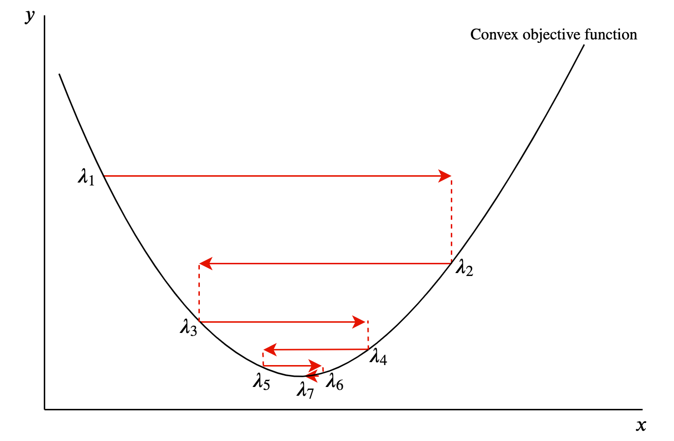
Figure 9.1: Gradient descent procedure in two dimensions.
PD matrices are like the parabola above. Geometrically, they are bowl-shaped and are guaranteed to have a global minimum.17 Consider rolling a ball on the inside surface of this bowl. It would run up and down the edges (losing height each time) before eventually resting on the bottom of the bowl, i.e. converging on the global minimum. Our algorithm is therefore bound to find the global minimum, and this is obviously a very useful property from an optimisation perspective.
If a matrix is PSD, on the other hand, we are not guaranteed to converge on a global minima. PSD matrices have “saddle points” where the slope is zero in all directions, but are neither (local) minima or maxima in all dimensions. Geometrically, for example, PSD matrices can look like hyperbolic parabaloids (shaped like a Pringles crisp). While there is a point on the surface that is flat in all dimensions, it may be a minima in one dimension, but a maxima in another.
PSD matrices prove more difficult to optimise because we are not guaranteed to converge on that point. At a point just away from the saddle point, we may actually want to move in opposite direction to the gradient dependent on the axis. In other words, the valence of the individual elements of the gradient vector point in different directions. Again, imagine dropping a ball onto the surface of a hyperbolic parabaloid. The ball is likely to pass the saddle point then run off one of the sides: gravity is pulling it down in to a minima in one dimension, but away from a maxima in another. PSD matrices therefore prove trickier to optimise, and can even mean we do not converge on a miniimum loss value. Therefore our stable of basic algorithms like GD like gradient descent are less likely to be effective optimisers.
9.3.3 Recap
In this final section, we have covered two applications of positive (semi-) definiteness: the proof of OLS as BLUE, and the ease of optimisation when a matrix is PD. There is clearly far more that can be discussed with respect to P(S)D matrices, and this chapter links or cites various resources that can be used to go further.
References
This short proof is taken from this discussion.↩︎
See these UPenn lecture notes for more details.↩︎