Chapter 3 Linear Projection
This chapter provides a basic introduction to projection using both linear algebra and geometric demonstrations. I discuss the derivation of the orthogonal projection, its general properties as an “operator”, and explore its relationship with ordinary least squares (OLS) regression. I defer a discussion of linear projections’ applications until the penultimate chapter on the Frisch-Waugh Theorem, where projection matrices feature heavily in the proof.
3.1 Projection
Formally, a projection \(P\) is a linear function on a vector space, such that when it is applied to itself you get the same result i.e. \(P^2 = P\).5
This definition is slightly intractable, but the intuition is reasonably simple. Consider a vector \(v\) in two-dimensions. \(v\) is a finite straight line pointing in a given direction. Suppose there is some point \(x\) not on this straight line but in the same two-dimensional space. The projection of \(x\), i.e. \(Px\), is a function that returns the point “closest” to \(x\) along the vector line \(v\). Call this point \(\bar{x}\). In most contexts, closest refers to Euclidean distance, i.e. \(\sqrt{\sum_{i} (x_i - \bar{x}_i)^2},\) where \(i\) ranges over the dimensions of the vector space (in this case two dimensions).6 Figure 3.1 depicts this logic visually. The green dashed line shows the orthogonal projection, and red dashed lines indicate other potential (non-orthgonal) projections that are further away in Euclidean space from \(x\) than \(\bar{x}\).
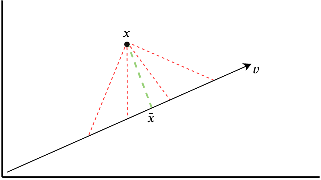
Figure 3.1: Orthogonal projection of a point onto a vector line.
In short, projection is a way of simplifying some n-dimensional space – compressing information onto a (hyper-) plane. This is useful especially in social science settings where the complexity of the phenomena we study mean exact prediction is impossible. Instead, we often want to construct models that compress busy and variable data into simpler, parsimonious explanations. Projection is the statistical method of achieving this – it takes the full space and simplifies it with respect to a certain number of dimensions.
While the above is (reasonably) intuitive it is worth spelling out the maths behind projection, not least because it helps demonstrate the connection between linear projection and linear regression.
To begin, we can take some point in n-dimensional space, \(x\), and the vector line \(v\) along which we want to project \(x\). The goal is the following:
\[ \begin{aligned} {arg\,min}_c \sqrt{\sum_{i} (\bar{x}_i - x)^2} & = {arg\,min}_c \sum_{i} (\bar{x}_i - x)^2 \\ & = {arg\,min}_c \sum_{i} (cv_i - x)^2 \end{aligned} \]
This rearrangement follows since the square root is a monotonic transformation, such that the optimal choice of \(c\) is the same across both \(arg\;min\)’s. Since any potential \(\bar{x}\) along the line drawn by \(v\) is some scalar multiplication of that line (\(cv\)), we can express the function to be minimised with respect to \(c\), and then differentiate:
\[ \begin{aligned} \frac{d}{dc} \sum_{i} (cv_i - x)^2 & = \sum_{i}2v_i(cv_i - x) \\ & = 2(\sum_{i}cv_i^2 - \sum_{i}v_ix) \\ & = 2(cv'v - v'x) \Rightarrow 0 \end{aligned} \]
Here we differentiate the equation and rearrange terms. The final step simply converts the summation notation into matrix multiplication. Solving:
\[ \begin{aligned} 2(cv'v - v'x) &= 0 \label{eq:dc_equal_zero} \\ cv'v - v'x &= 0 \\ cv'v &= v'x \\ c &= (v'v)^{-1}v'x. \end{aligned} \]
From here, note that \(\bar{x}\), the projection of \(x\) onto the vector line, is \(vc = v(v'v)^{-1}v'x.\) Hence, we can define the projection matrix of \(x\) onto \(v\) as:
\[ P_v = v(v'v)^{-1}v'.\]
In plain English, for any point in some space, the orthogonal projection of that point onto some subspace, is the point on a vector line that minimises the Euclidian distance between itself and the original point. A visual demonstration of this point is shown and discussed in Figure 3.3 below.
Note also that this projection matrix has a clear analogue to the linear algebraic expression of linear regression. The vector of coefficients in a linear regression \(\hat{\beta}\) can be expressed as \((X′X)^{-1}X′y\). And we know that multiplying this vector by the matrix of predictors \(X\) results in the vector of predicted values \(\hat{y}\). Now we have \(\hat{y} = X(X'X)^{-1}X'Y \equiv P_Xy\). Clearly, therefore, linear projection and linear regression are closely related – and I return to this point below.
3.2 Properties of the projection matrix
The projection matrix \(P\) has several interesting properties. First, and most simply, the projection matrix is square. Since \(v\) is of some arbitrary dimensions \(n \times k\), its transpose is of dimensions \(k \times n\). By linear algebra, the shape of the full matrix is therefore \(n \times n\), i.e. square.
Projection matrices are also symmetric, i.e. \(P = P'\). To prove symmetry, note that transposing both sides of the projection matrix definition:
\[\begin{align} P' &= (v(v'v)^{-1}v')' \\ &= v(v'v)^{-1}v'\\ &= P, \end{align}\]
since \((AB)'=B'A'\) and \((A^{-1})' = (A')^{-1}.\)
Projection matrices are idempotent:
\[\begin{align} PP &= v(v'v)^{-1}v'v(v'v)^{-1}v' \\ &= v(v'v)^{-1}v'\\ &= P, \end{align}\]
since \((A)^{-1}A = I\) and \(BI = B\).
Since, projection matrices are idempotent, this entails that projecting a point already on the vector line will just return that same point. This is fairly intuitive: the closest point on the vector line to a point already on the vector line is just that same point.
Finally, we can see that the projection of any point is orthogonal to the respected projected point on vector line. Two vectors are orthogonal if \(ab = 0\). Starting with the expression for the derivative we found earlier (i.e. minimising the Euclidean distance with respect to \(c\)):
\[ \begin{aligned} 2(cv'v - v'x) &= 0 \\ v'cv - v'x &= 0 \\ v'(cv-x) &= 0 \\ v'(\bar{x} - x) &= 0, \end{aligned} \]
hence the line connecting the original point \(x\) is orthogonal to the vector line.
The projection matrix is very useful in other fundamental theorems in econometrics, like Frisch Waugh Lovell Theorem discussed in Chapter 8.
3.3 Linear regression
Given a vector of interest, how do we capture as much information from it as possible using set of predictors? Projection matrices essentially simplify the dimensionality of some space, by casting points onto a lower-dimensional plane. Think of it like capturing the shadow of an object on the ground. There is far more detail in the actual object itself but we roughly know its position, shape, and scale from the shadow that’s cast on the 2d plane of the ground.
Note also this is actually quite similar to how we think about regression. Loosely, when we regress \(Y\) on \(X\), we are trying to characterise how the components (or predictors) within \(X\) characterise or relate to \(Y\). Of course, regression is also imperfect (after all, the optimisation goal is to minimise the errors of our predictions). So, regression also seems to capture some lower dimensional approximation of an outcome.
In fact, linear projection and linear regression are very closely related. In this final section, I outline how these two statistical concepts relate to each other, both algebraically and geometrically,
Suppose we have a vector of outcomes \(y\), and some n-dimensional matrix \(X\) of predictors. We write the linear regression model as:
\[\begin{equation} y = X\beta + \epsilon, \end{equation}\]
where \(\beta\) is a vector of coefficients, and \(\epsilon\) is the difference between the prediction and the observed value in \(y\). The goal of linear regression is to minimise the sum of the squared residuals:
\[ arg\,min \,\, \epsilon^2 = arg\,min (y - X\beta)'(y-X\beta) \]
Differentiating with respect to and solving: \[ \begin{aligned} \frac{d}{d\beta} (y - X\beta)'(y-X\beta) &= -2X(y - X\beta) \\ &= 2X'X\beta -2X'y \Rightarrow 0 \\ X'X\hat{\beta} &= X'y \\ (X'X)^{-1}X'X\hat{\beta} &= (X'X)^{-1}X'y \\ \hat{\beta} &= (X'X)^{-1}X'y. \end{aligned} \]
To get our prediction of \(y\), i.e. \(\hat{y}\), we simply multiply our beta coefficient by the matrix X:
\[ \hat{y} = X(X'X)^{-1}X'y. \]
Note how the OLS derivation of \(\hat{y}\) is very similar to \(P = X(X'X)^{-1}X\), the orthogonal prediction matrix. The two differ only in that that \(\hat{y}\) includes the original outcome vector \(y\) in its expression. But, note that \(Py = X(X'X)^{-1}X'y = \hat{y}\)! Hence the predicted values from a linear regression simply are an orthogonal projection of \(y\) onto the space defined by \(X\).
3.3.1 Geometric interpretation
It should be clear now that linear projection and linear regression are connected – but it is probably less clear why this holds. To understand what’s going on, let’s depict the problem geometrically.7
To appreciate what’s going on, we first need to invert how we typically think about observations, variables and datapoints. Consider a bivariate regression problem with three observations. Our data will include three variables: a constant (c, a vector of 1’s), a predictor (X), and an outcome variable (Y). As a matrix, this might look something like the following:
| Y | X | c |
|---|---|---|
| 2 | 3 | 1 |
| 3 | 1 | 1 |
| 2 | 1 | 1 |
Typically we would represent the relationship geometrically by treating the variables as dimensions, such that every datapoint is an observation (and we would typically ignore the constant column since all its values are the same).
An alternative way to represent this data is to treat each observation (i.e. row) as a dimension and then represent each variable as a vector. What does that actually mean? Well consider the column \(Y = (2,3,2)\). This vector essentially gives us the coordinates for a point in three-dimensional space: \(d_1 = 2, d_2 = 3, d_3 = 2\). Drawing a straight line from the origin (0,0,0) to this point gives us a vector line for the outcome. While visually this might seem strange, from the perspective of our data it’s not unusual to refer to each variable as a column vector, and that’s precisely because it is a quantity with a magnitude and direction (as determined by its position in \(n\) dimensions).
Our predictors are the vectors \(X\) and \(c\) (note the vector \(c\) is now slightly more interesting because it is a diagonal line through the three-dimensional space). We can extend either vector line by multiplying it by a constant e.g. \(2X = (6,2,2)\). With a single vector, we can only move forwards or backwards along a line. But if we combine two vectors together, we can actually reach lots of points in space. Imagine placing the vector \(X\) at the end of the \(c\). The total path now reaches a new point that is not intersected by either \(X\) or \(c\). In fact, if we multiply \(X\) and \(c\) by some scalars (numbers), we can snake our way across a whole array of different points in three-dimensional space. Figure 3.2 demonstrates some of these combinations in the two dimensional space created by \(X\) and \(c\).
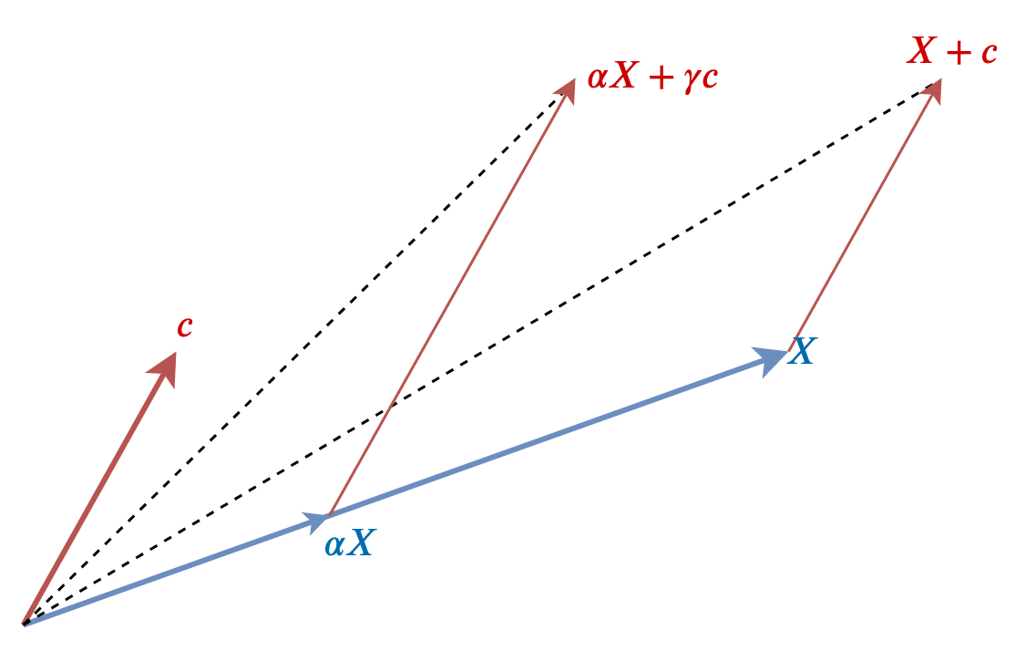
Figure 3.2: Potential combinations of two vectors.
The comprehensive set of all possible points covered by linear combinations of \(X\) and \(c\) is called the span or column space. In fact, with the specific set up of this example (3 observations, two predictors), the span of our predictors is a flat plane. Imagine taking a flat bit of paper and aligning one corner with the origin, and then angling surface so that the end points of the vectors \(X\) and \(c\) are both resting on the card’s surface. Keeping that alignment, any point on the surface of the card is reachable by some combination of \(X\) and \(c\). Algebraically we can refer to this surface as \(col(X,c)\), and it generalises beyond two predictors (although this is much harder to visualise).
Crucially, in our reduced example of three-dimensional space, there are points in space not reachable by combining these two vectors (any point above or below the piece of card). We know, for instance that the vector line \(y\) lies off this plane. The goal therefore is to find a vector that is on the column space of \((X,c)\) that gets closest to our off-plane vector \(y\) as possible. Figure 3.3 depicts this set up visually – each dimension is an observation, each column in the matrix is represented a vector, and the column space of \((X,c)\) is the shaded grey plane. The vector \(y\) lies off this plane.
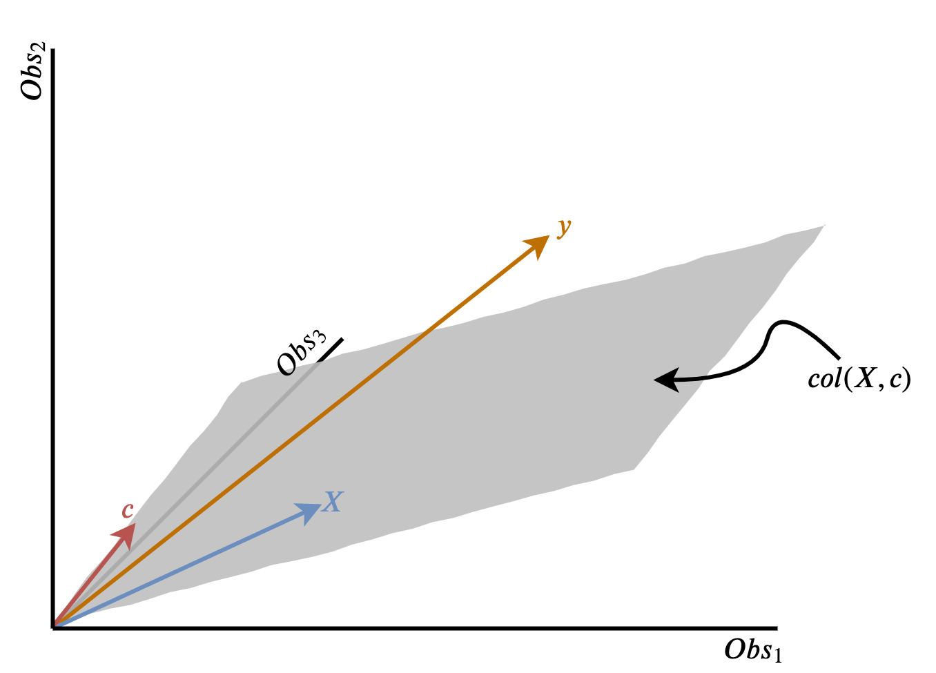
Figure 3.3: Schematic of orthogonal projection as a geometric problem
From our discussion in Section 3.1, we know that the “best” vector is the orthogonal projection from the column space to the vector \(y\). This is the shortest possible distance between the flat plane and the observed outcome, and is just \(\hat{y}\). Moreover, since \(\hat{y}\) lies on the column space, we know we only need to combine some scaled amount of \(X\) and \(c\) to define the vector \(\hat{y}\), i.e., \(\beta_1X + \beta_0c\). Figure 3.4 shows this geometrically. And in fact, the scalar coefficients \(\beta_1, \beta_0\) in this case are just the regression coefficients derived from OLS. Why? Because we know that the orthogonal projection of \(y\) onto the column space minimises the error between our prediction \(\hat{y}\) and the observed outcome vector \(y\). This is the same as the minimisation problem that OLS solves, as outlined at the beginning of this section!
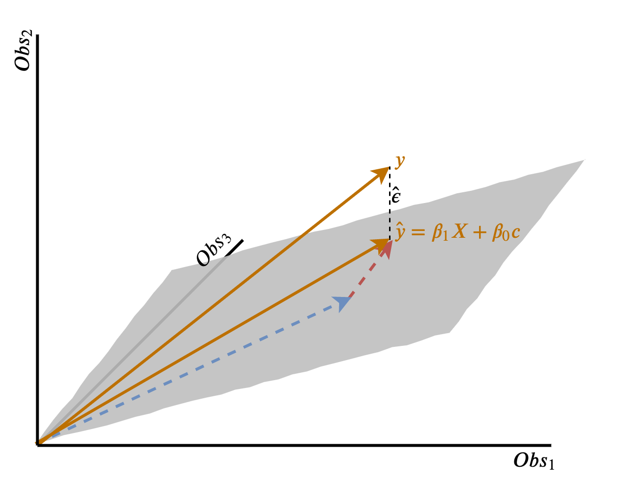
Figure 3.4: Relation of orthogonal projection to linear regression.
Consider any other vector on the column space, and the distance between itself and and \(y\). Each non-orthogonal vector would be longer, and hence have a larger predictive error, than \(\hat{y}\). For example, Figure 3.5 plots two alternative vectors on \(col(X,c)\) alongside \(\hat{y}\). Clearly, \(\hat{\epsilon} < \epsilon' < \epsilon'',\) and this is true of any other vector on the column space too.
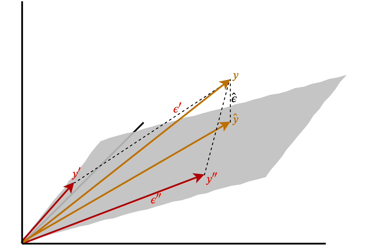
Figure 3.5: Alternative vectors on the column space are further away from y.
Hence, linear projection and linear regression can be seen (both algebraically and geometrically) to be solving the same problem – minimising the (squared) distance between an observed vector \(y\) and prediction vector \(\hat{y}\). This demonstration generalises to many dimensions (observations), though of course it becomes much harder to intuit the geometry of highly-dimensional data. And similarly, with more observations we could also extend the number of predictors too such that \(X\) is not a single column vector but a matrix of predictor variables (i.e. multivariate regression). Again, visualising what the column space of this matrix would look like geometrically becomes harder.
To summarise, this section has demonstrated two features. First, that linear regression simply is an orthogonal projection. We saw this algebraically by noting that the derivation of OLS coefficients, and subsequently the predicted values from a linear regression, is identical to \(Py\) (where \(P\) is a projection matrix). Second, and geometrically, we intuited why this is the case: namely that projecting onto a lower-dimensional column space involves finding the linear combination of predictors that minimises the Euclidean distance to \(y\), i.e. \(\hat{y}\). The scalars we use to do so are simply the regression coefficients we would generate using OLS regression.
Since \(P\) is (in the finite case) a square matrix, a projection matrix is an idempotent matrix – I discuss this property in more detail later on in this note.↩︎
Euclidean distance has convenient properties, including that the closest distance between a point and a vector line is orthogonal to the vector line itself.↩︎
This final section borrows heavily from Ben Lambert’s explanation of projection and a demonstration using R by Andy Eggers.↩︎