2 K-nearest Neighbours Regression

2.1 Introduction

KNN regression is a non-parametric method that, in an intuitive manner, approximates the association between independent variables and the continuous outcome by averaging the observations in the same neighbourhood. The size of the neighbourhood needs to be set by the analyst or can be chosen using cross-validation (we will see this later) to select the size that minimises the mean-squared error.

While the method is quite appealing, it quickly becomes impractical when the dimension increases, i.e., when there are many independent variables.

2.2 Readings

Read the following chapter of An introduction to statistical learning:

• 3.5 Comparison of Linear Regression with K-Nearest Neighbors

2.3 Practical session

TASK - Fit a knn regression

With the bmd.csv dataset, we want to fit a knn regression with k=3 for BMD, with age as covariates. Then we will compute the MSE and \(R^2\).

#libraries that we will need
library(FNN)   #knn regression
set.seed(1974) #fix the random generator seed 

#read the data
bmd.data     <- 
  read.csv("https://www.dropbox.com/s/c6mhgatkotuze8o/bmd.csv?dl=1", 
           stringsAsFactors = TRUE)

#Fit a knn regression with k=3
#using the knn.reg() function from the FNN package
knn3.bmd <- knn.reg(train=bmd.data[c("age")],   
                     y=bmd.data$bmd, 
                     test= data.frame(age=seq(38,89)),
                     k=3)    

Before computing the MSE and \(R^2\), we will plot the model predictions

  plot(bmd.data$age, bmd.data$bmd) #adding the scatter for BMI and BMD
  lines(seq(38,89), knn3.bmd$pred)  #adds the knn k=3 line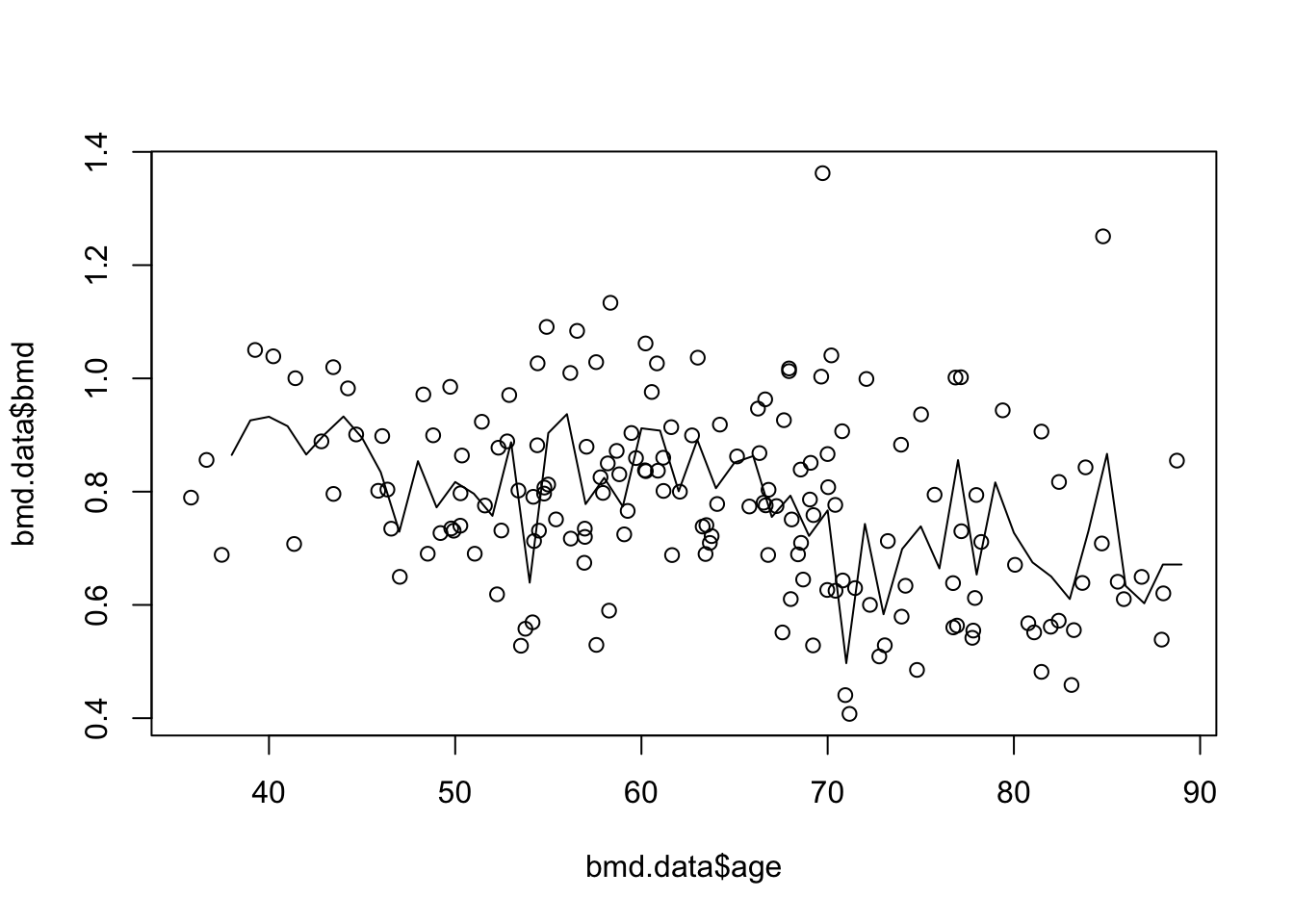

Finally, we compute the MSE and \(R^2\) for knn k=3. We have to refit the models and “test” them in the original data

  knn3.bmd.datapred <- knn.reg(train=bmd.data[c("age")],  
                           y=bmd.data$bmd, 
                           test=bmd.data[c("age")], #ORIGINAL DATA
                           k=3)      #knn reg with k=3
  #MSE for knn k=3 
  mse.knn3  <- mean((knn3.bmd.datapred$pred - bmd.data$bmd)^2)  
  mse.knn3

## [1] 0.01531282

  r2.knn3   <- 1- mse.knn3/(var(bmd.data$bmd)*168/169) #R2 for knn k=3 using 
  r2.knn3                                              #R2 = 1-MSE/var(y)

## [1] 0.4445392

TRY IT YOURSELF:

1. Fit a knn regression for BMD using AGE, with k=20

See the solution code

  knn20.bmd <- knn.reg(train=bmd.data[c("age")],   
                      y=bmd.data$bmd, 
                      test= data.frame(age=seq(38,89)),
                      k=20)     #knn regression with k=20

2. Add the prediction line to the previous scatter plot

See the solution code

plot(bmd.data$age, bmd.data$bmd) #adding the scatter for BMI and BMD
lines(seq(38,89), knn3.bmd$pred) 
lines(seq(38,89), knn20.bmd$pred, col="blue")  #adds the knn k=20 gray line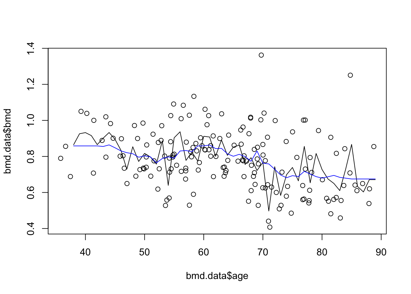

3. Compute the MSE and \(R^2\)

See the solution code

#predictions from knn reg with k=20
knn20.bmd.datapred <- knn.reg(
  train = bmd.data[c("age")],
  y = bmd.data$bmd,
  test = bmd.data[c("age")],
  #ORIGINAL DATA
  k = 20
)    

#MSE for knn k=20
mse.knn20 <- mean((knn20.bmd.datapred$pred - bmd.data$bmd) ^ 2) 
mse.knn20

#r2 for knn k=20
r2.knn20 <- 1-mse.knn20/(var(bmd.data$bmd)*168/169) #168/169 is added to correct 
r2.knn20                                              #the degrees of freedom

4. Add a linear prediction for BMD using AGE to the scatter plot

See the solution code

#The initial plot with knn3 and knn20
plot(bmd.data$age, bmd.data$bmd) #adding the scatter for BMI and BMD
lines(seq(38,89), knn3.bmd$pred) 
lines(seq(38,89), knn20.bmd$pred, col="blue")  #adds the knn k=20 gray line
  
#linear model and predictions  
model.age <- lm(bmd ~ age, 
                   data = bmd.data)
bmd.pred <- predict(model.age, 
                   newdata = data.frame(age=seq(38,89)))
lines(seq(38,89), bmd.pred) #add the linear predictions to the plot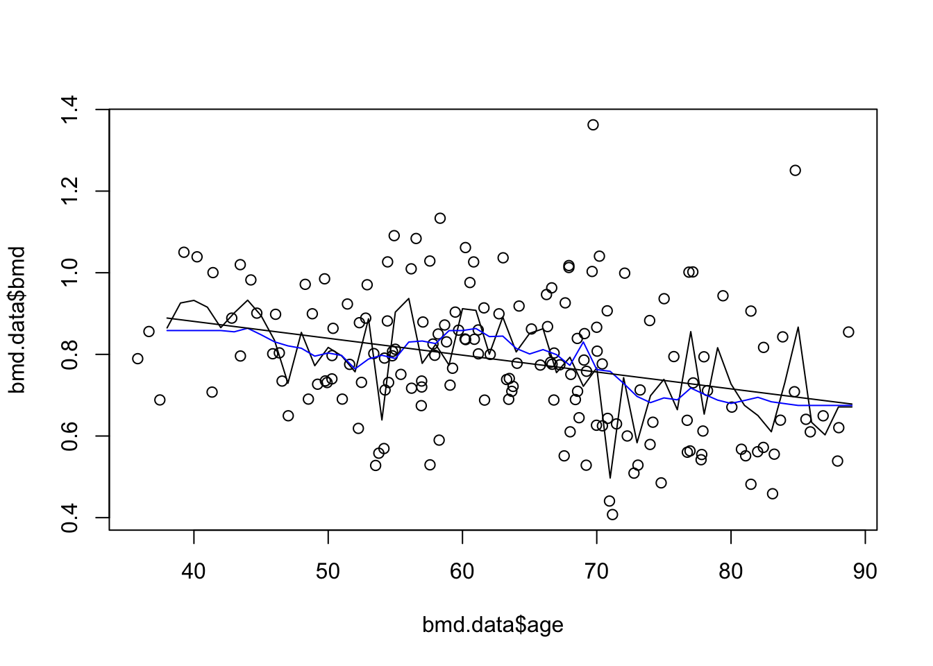

2.4 Exercises

1. With the fat dataset in the library(faraway), we want to predict body fat (variable brozek) using the variable abdom

   1. use a k-nearest neighbour regression, with k=3,5 and 11, to approximate the relation between brozek and abdom. Plot the three lines.

   2. What is the predicted brozek for someone with abdom=90 using knn=11?

   3. What is the predicted brozek for someone with abdom=90 using a linear model?

   4. Compute the mean squared error for k=3,5 and 11

2. With the same data fat, use a knn (k=9) to predict body fat (variable brozek) using the variables abdom and age

1. Plot the predictions for abdom = 80 to 115 and age = 30

2. Would you expect the mean squared error for k=1 to be greater or smaller than the one for k=9? Why would you prefer k=9 over k=1?