5 K-nearest Neighbours Classification
5.1 Introduction
The K-nearest Neighbours (KNN) for classification, uses a similar idea to the KNN regression. For KNN, a unit will be classified as the majority of its neighbours.
5.2 Readings
Read the following chapters of An introduction to statistical learning:
- 4.1 An Overview of Classification
- 2.2.3 The Classification Setting
5.3 Practical session
TASK - KNN classification
With the bmd.csv dataset, we will use KNN (k=3) with the variables AGE, SEX, BMI and BMD to classify FRACTURE and compute the confusion matrix
First, let’s import the dataset
#libraries that we will need
library(class)   #knn
set.seed(1974) #fix the random generator seed

#read the data
bmd.data     <-
  read.csv("https://www.dropbox.com/s/c6mhgatkotuze8o/bmd.csv?dl=1",
           stringsAsFactors = TRUE)

bmd.data$bmi <- bmd.data$weight_kg / (bmd.data$height_cm/100)^2
let’s standardise all the variables so they have mean 0 and SD=1 so that the distances are in the same scale.
  bmd.data$age.std     <- scale(bmd.data$age)
  bmd.data$sex.num.std <- scale(as.numeric(bmd.data$sex)) #1-F, #2-M
  bmd.data$bmi.std     <- scale(bmd.data$bmi)
  bmd.data$bmd.std     <- scale(bmd.data$bmd)
Now we use knn=3
model.knn3 <-  knn(train = bmd.data[c("age.std", "sex.num.std",
                                      "bmi.std","bmd.std")],
                   test  = bmd.data[c("age.std", "sex.num.std",
                                      "bmi.std","bmd.std")],
                    cl    = bmd.data$fracture, k=3)
table(model.knn3, bmd.data$fracture)
##
## model.knn3 fracture no fracture
## fracture 38 7
## no fracture 12 112TRY IT YOURSELF:
- Repeat the classification model from above but now with k=20 and compute the confusion matrix.
See the solution code
  model.knn20 <-  knn(train = bmd.data[c("age.std", "sex.num.std",
                                        "bmi.std","bmd.std")],
                   test  = bmd.data[c("age.std", "sex.num.std",
                                         "bmi.std","bmd.std")],
                    cl    = bmd.data$fracture, k=20 )
  table(model.knn20, bmd.data$fracture)
- (hard) Plot the error rate for KNN with k=1 to 20 using the variables AGE, SEX, BMI and BMD to classify FRACTURE
See the solution code
knn.fit <- function(k.par){
  knn.model <- knn(train = bmd.data[c("age.std", "sex.num.std",
                                      "bmi.std","bmd.std")],
                   test  = bmd.data[c("age.std", "sex.num.std",
                                      "bmi.std","bmd.std")],
                    cl    = bmd.data$fracture, k=k.par )
  class.error<- 1-sum(diag(table( knn.model, bmd.data$fracture))/169)
  return(class.error)
}

  class.error1to20 <- sapply(seq(1,20), knn.fit)
  plot(seq(1,20), class.error1to20, type="l")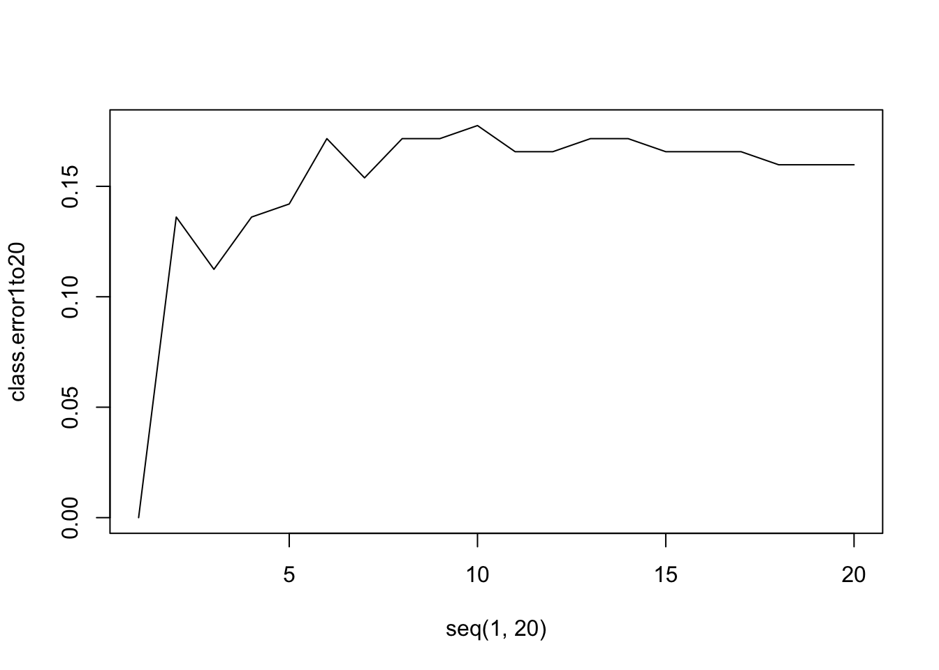
5.4 Exercises
The dataset bdiag.csv, included several imaging details from patients that had a biopsy to test for breast cancer.
The variable diagnosis classifies the biopsied tissue as M = malignant or B = benign.Use a KNN with k=5 to predict Diagnosis using texture_mean and radius_mean.
Build the confusion matrix for the classification above
Plot the scatter plot for texture_mean and radius_mean and draw the border line for the prediction of Diagnosis based on the model in a)
Plot the scatter plot for texture_mean and radius_mean and draw the border line for the prediction of Diagnosis based knn, k=15