Chapter 9 Class 8 20 10 2020 - t-test and ANOVA are just linear models

The objective of this chapter is to explore different regression models and to see how they relate to statistical procedures one might not associate with a regression, when in fact, they are just special cases of a regression.

9.1 The t-test

While we did not do the t-test in class, this is useful because it allows you to see how a simple t-test is just a linear model too, and acts as a building block for the next examples. The t-test allows us to test the null hypothesis that two samples have the same mean.

Create some data

#Making up a t-test
#making sure everyone gets the same results
set.seed(980)

Then we define the sample size and the number of treatments

#define sample size
n=100
#define treatments
tr=c("a","b")
#how many treatments - 2 for a t test
ntr=length(tr)
#balanced design
n.by.tr=n/ntr

Now, we can simulate some data. First, the treatments

type=as.factor(rep(tr,each=n.by.tr))
cores=rep(1:ntr,each=n.by.tr)

Then we define the means by treatment - note that they are different, so the null hypothesis in the t-test, that the mean of a is equal to the mean of b, is known to be false in this case.

#define 4 means
ms=c(3,4)

Then, the key part, the response variable, with a different mean by treatment. Note the use of the ifelse function, which evaluates its first argument and then assigns the value of its second argument if the first is true or the value of the second if its first argument is false. An example

ifelse(3>4,55,77)

## [1] 77

ifelse(3<4,55,77)

## [1] 55

So now, generate the response data

ys=ifelse(type=="a",ms[1],ms[2])+rnorm(n,0,1.5)

Look at the data

plot(ys~type)

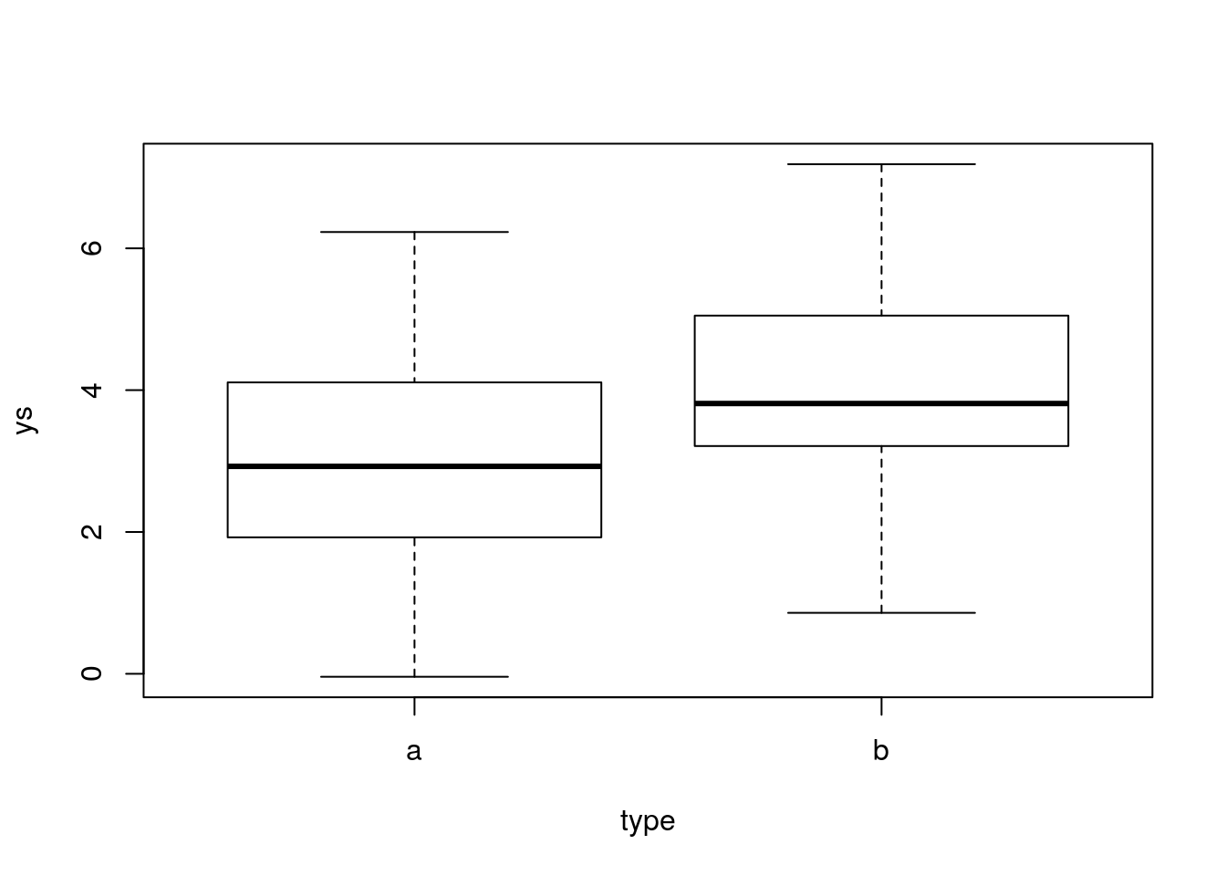
Now, we can run the usual t-test

t.test(ys~type)

## 
## 	Welch Two Sample t-test
## 
## data:  ys by type
## t = -2.8043, df = 97.475, p-value = 0.006087
## alternative hypothesis: true difference in means is not equal to 0
## 95 percent confidence interval:
##  -1.4263293 -0.2441277
## sample estimates:
## mean in group a mean in group b 
##        3.106656        3.941884

and now we can do it the linear regression way

lm0=lm(ys~type)
summary(lm0)

## 
## Call:
## lm(formula = ys ~ type)
## 
## Residuals:
##     Min      1Q  Median      3Q     Max 
## -3.1489 -0.9131 -0.1315  1.0295  3.2450 
## 
## Coefficients:
##             Estimate Std. Error t value Pr(>|t|)    
## (Intercept)   3.1067     0.2106  14.751  < 2e-16 ***
## typeb         0.8352     0.2978   2.804  0.00608 ** 
## ---
## Signif. codes:  0 '***' 0.001 '**' 0.01 '*' 0.05 '.' 0.1 ' ' 1
## 
## Residual standard error: 1.489 on 98 degrees of freedom
## Multiple R-squared:  0.07428,	Adjusted R-squared:  0.06484 
## F-statistic: 7.864 on 1 and 98 DF,  p-value: 0.006081

and as you can see, we get the same result for the test statistic. It is the same thing! And we can naturally get the estimated means per group. The mean for a is just the intercept of the model. To get the mean of the group b we add the mean of group b to the intercept, as

#mean of ys under treatment a
summary(lm0)$coefficients[1]

## [1] 3.106656

#mean of ys under treatment b
summary(lm0)$coefficients[1]+lm0$coefficients[2]

##    typeb 
## 3.941884

This is required because in a linear model, all the other parameters associated with levels of a factor will be compared to a reference value, that of the intercept, which happens to be the mean under treatment a. Below you will see more examples of this.

Note we were able to detect the null was false, but this was because we had a decent sample size compared to the variance of the measurements and the magnitude of the true effect (the difference of the means). If we keep the sample size constant but we increase the noise or decrease the magnitude of the difference, we might not get the same result, and make a type II error!

#define 2 means
ms=c(3,4)
#increase the variance of the process
ys=ifelse(type=="a",ms[1],ms[2])+rnorm(n,0,5)

Look at the data, we can see much more variation

plot(ys~type)

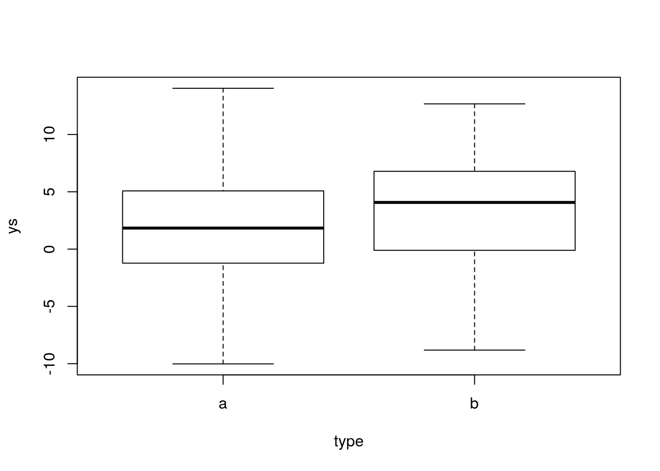
Now, we can run the usual t-test

t.test(ys~type)

## 
## 	Welch Two Sample t-test
## 
## data:  ys by type
## t = -1.3609, df = 97.949, p-value = 0.1767
## alternative hypothesis: true difference in means is not equal to 0
## 95 percent confidence interval:
##  -3.2822693  0.6118174
## sample estimates:
## mean in group a mean in group b 
##        2.024963        3.360189

and now we can do it the linear regression way

lm0=lm(ys~type)
summary(lm0)

## 
## Call:
## lm(formula = ys ~ type)
## 
## Residuals:
##      Min       1Q   Median       3Q      Max 
## -12.1746  -3.2719   0.2527   3.0578  12.0085 
## 
## Coefficients:
##             Estimate Std. Error t value Pr(>|t|)   
## (Intercept)   2.0250     0.6938   2.919  0.00436 **
## typeb         1.3352     0.9811   1.361  0.17667   
## ---
## Signif. codes:  0 '***' 0.001 '**' 0.01 '*' 0.05 '.' 0.1 ' ' 1
## 
## Residual standard error: 4.906 on 98 degrees of freedom
## Multiple R-squared:  0.01855,	Adjusted R-squared:  0.008533 
## F-statistic: 1.852 on 1 and 98 DF,  p-value: 0.1767

and as you can see, we get the same result for the test statistic, but now with a non significant test.

The same would have happened if we decreased the true difference, while keeping the original magnitude of the error

#define 2 means
ms=c(3,3.1)
#increase the variance of the process
ys=ifelse(type=="a",ms[1],ms[2])+rnorm(n,0,1.5)

Look at the data, we can see again lower variation, but the difference across treatments is very small (so, hard to detect!)

plot(ys~type)

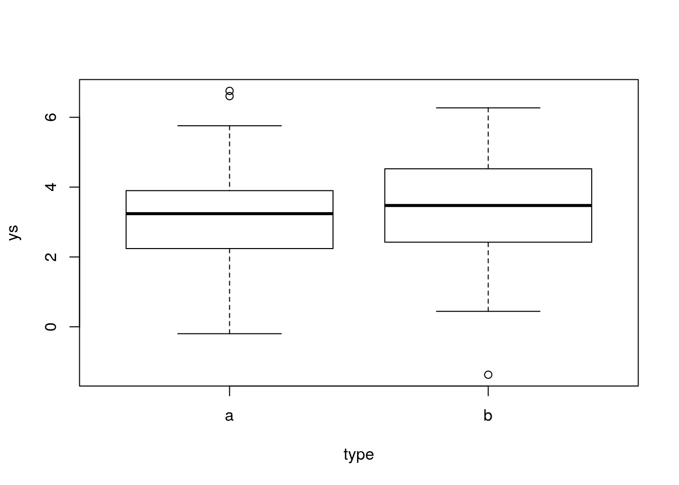
Now, we can run the usual t-test

t.test(ys~type)

## 
## 	Welch Two Sample t-test
## 
## data:  ys by type
## t = -0.7994, df = 97.455, p-value = 0.426
## alternative hypothesis: true difference in means is not equal to 0
## 95 percent confidence interval:
##  -0.8149517  0.3469402
## sample estimates:
## mean in group a mean in group b 
##        3.158868        3.392874

and now we can do it the linear regression way

lm0=lm(ys~type)
summary(lm0)

## 
## Call:
## lm(formula = ys ~ type)
## 
## Residuals:
##     Min      1Q  Median      3Q     Max 
## -4.7661 -0.9318  0.0812  0.9087  3.5981 
## 
## Coefficients:
##             Estimate Std. Error t value Pr(>|t|)    
## (Intercept)   3.1589     0.2070  15.261   <2e-16 ***
## typeb         0.2340     0.2927   0.799    0.426    
## ---
## Signif. codes:  0 '***' 0.001 '**' 0.01 '*' 0.05 '.' 0.1 ' ' 1
## 
## Residual standard error: 1.464 on 98 degrees of freedom
## Multiple R-squared:  0.006479,	Adjusted R-squared:  -0.003659 
## F-statistic: 0.639 on 1 and 98 DF,  p-value: 0.426

9.2 ANOVA

We move on with perhaps the most famous example of a statistical test/procedure, the ANOVA. An ANOVA is nothing but a linear model, where we have a continuous response variable, which we want to explain as a function of a factor (with several levels, or treatments).

We simulate a data set, beginning by making sure everyone gets the same results by using set.seed

#Making up an ANOVA
#An ANOVA
#making sure everyone gets the same results
set.seed(12345)

Then we define the sample size and the number of treatments

#define sample size
n=2000
#define treatments
tr=c("a","b","c","d")
#how many treatments
ntr=length(tr)
#balanced design
n.by.tr=n/ntr

now, we can simulate some data. First, the treatments, but we also generate a independent variable that is not really used for now (xs).

#generate data
xs=runif(n,10,20)
type=as.factor(rep(tr,each=n.by.tr))
#if I wanted to recode the levels such that c was the baseline
#type=factor(type,levels = c("c","a","b","d"))
#get colors for plotting
cores=rep(1:ntr,each=n.by.tr)

Then we define the means by treatment - note that they are different, so the null hypothesis in an ANOVA, that all the means are the same, is false.

#define 4 means
ms=c(3,5,6,2)

ifelse(3>4,55,77)

## [1] 77

ifelse(3<4,55,77)

## [1] 55

Note these can be used nested, leading to possible multiple outcomes, and I use that below to define 4 different means depending on the treatment of the observation

ifelse(3<4,55,ifelse(3>2,55,68))

## [1] 55

ifelse(3>4,55,ifelse(3>2,666,68))

## [1] 666

ifelse(3>4,55,ifelse(3<2,666,68))

## [1] 68

So now, generate the data

#ys, not a function of the xs!!!
ys=ifelse(type=="a",ms[1],ifelse(type=="b",ms[2],ifelse(type=="c",ms[3],ms[4])))+rnorm(n,0,3)

We can actually look at the simulated data

par(mfrow=c(1,1),mar=c(4,4,0.5,0.5))
plot(ys~type,col=1:4)

#abline(h=ms,col=1:4)

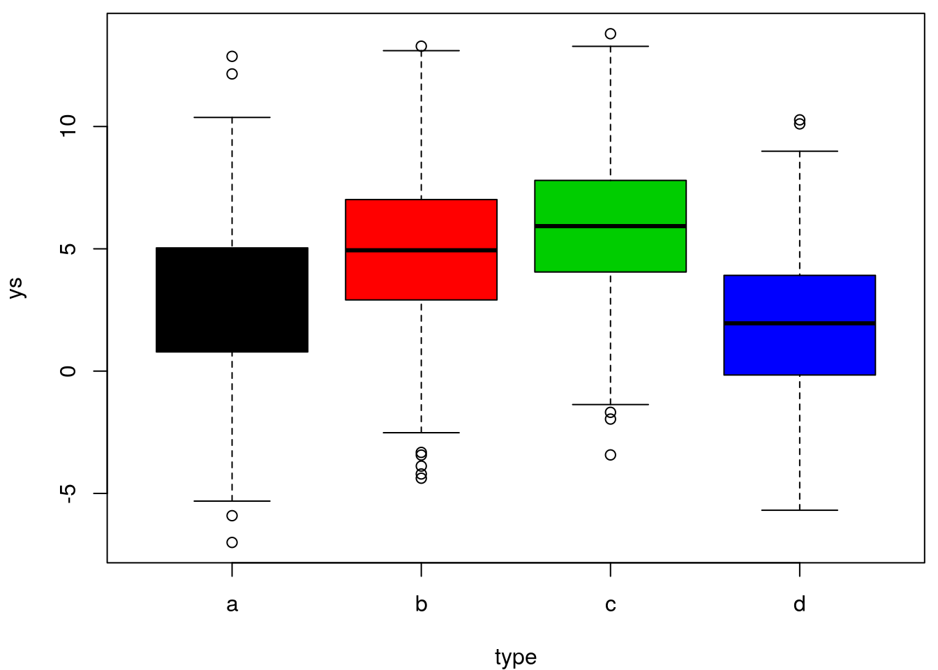
finally, we can implement the linear model and look at its summary

lm.anova=lm(ys~type)
summary(lm.anova)

## 
## Call:
## lm(formula = ys ~ type)
## 
## Residuals:
##     Min      1Q  Median      3Q     Max 
## -9.8735 -2.0115  0.0301  2.0208  9.9976 
## 
## Coefficients:
##             Estimate Std. Error t value Pr(>|t|)    
## (Intercept)   2.8694     0.1319  21.753  < 2e-16 ***
## typeb         2.0788     0.1865  11.143  < 2e-16 ***
## typec         2.9806     0.1865  15.978  < 2e-16 ***
## typed        -0.8726     0.1865  -4.678 3.09e-06 ***
## ---
## Signif. codes:  0 '***' 0.001 '**' 0.01 '*' 0.05 '.' 0.1 ' ' 1
## 
## Residual standard error: 2.95 on 1996 degrees of freedom
## Multiple R-squared:  0.2163,	Adjusted R-squared:  0.2151 
## F-statistic: 183.6 on 3 and 1996 DF,  p-value: < 2.2e-16

note that, again, we can manipulate any sub-components of the created objects

#see the parameters
lm.anova$coefficients

## (Intercept)       typeb       typec       typed 
##   2.8694412   2.0787628   2.9806367  -0.8726428

#see the third parameter
lm.anova$coefficients[3]

##    typec 
## 2.980637

Not surprisingly, because the means were different and we had a large sample size, everything is highly significant. Note that the ANOVA test is actually presented in the regression output, and that is the corresponding F-test

summary(lm.anova)$fstatistic

##     value     numdf     dendf 
##  183.6156    3.0000 1996.0000

and we can use the F distribution to calculate the corresponding P-value (note that is already in the output above)

ftest=summary(lm.anova)$fstatistic[1]
df1=summary(lm.anova)$fstatistic[2]
df2=summary(lm.anova)$fstatistic[3]
pt(ftest,df1,df2)

##         value 
## 1.402786e-131

OK, this is actually the exact value, while above the value was reported as just a small value (< 2.2 \(\times\) 10\(^{-16}\)), but it is the same value, believe me!

Finally, to show (by example) this is just what the ANOVA does, we have the NAOVA itself

summary(aov(lm.anova))

##               Df Sum Sq Mean Sq F value Pr(>F)    
## type           3   4792  1597.5   183.6 <2e-16 ***
## Residuals   1996  17365     8.7                   
## ---
## Signif. codes:  0 '***' 0.001 '**' 0.01 '*' 0.05 '.' 0.1 ' ' 1

where everything is the same (test statistic, degrees of freedom and p-values).

Conclusion: an ANOVA is just a special case of a linear model, one where we have a continuous response variable and a factor explanatory covariate. In fact, a two way ANOVA is just the extension where we have a continuous response variable and 2 factor explanatory covariates, and, you guessed it, a three way ANOVA means we have a continuous response variable and a 3 factor explanatory covariates.

Just to finish up this example, we could now plot the true means per treatment, the estimated means per treatment

par(mfrow=c(1,1),mar=c(4,4,0.5,0.5))
plot(as.numeric(type),ys,col=as.numeric(type),xlab="Treatment",xaxt="n")
axis(1,at=1:4,letters[1:4])
#plot the estimated line for type a
abline(h=lm.anova$coefficients[1],lwd=3,col=1)
#plot the mean line for type a
abline(h=mean(ys[type=="a"]),lwd=1,col=1,lty=2)
#plot the real mean for type a
abline(h=ms[1],lwd=2,col=1,lty=3)
#and now for the other types
abline(h=lm.anova$coefficients[1]+lm.anova$coefficients[2],lwd=3,col=2)
abline(h=mean(ys[type=="b"]),lwd=1,col=2,lty=2)
#plot the real mean for type b
abline(h=ms[2],lwd=2,col=2,lty=3)
abline(h=lm.anova$coefficients[1]+lm.anova$coefficients[3],lwd=3,col=3)
abline(h=mean(ys[type=="c"]),lwd=1,col=3,lty=2)
#plot the real mean for type c
abline(h=ms[3],lwd=2,col=3,lty=3)
abline(h=lm.anova$coefficients[1]+lm.anova$coefficients[4],lwd=3,col=4)
abline(h=mean(ys[type=="d"]),lwd=1,col=4,lty=2)
#plot the real mean for type a
abline(h=ms[4],lwd=2,col=4,lty=3)
legend("topright",c("Estimated","Mean of data","True"),lwd=c(4,1,2),lty=c(1,3,2),inset=0.03)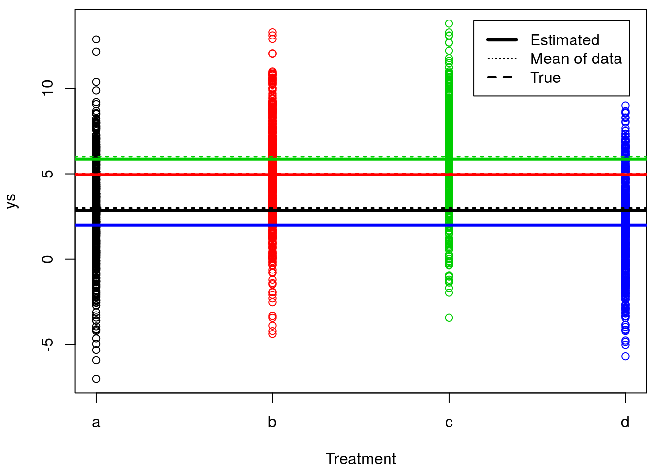

It’s not easy to see because these overlap (large sample size, high precision) but the estimated means are really close to the real means. It’s a bit easier to see if we separate in 4 plots and zoom in on the mean of each treatment, but still the blue lines are all on top of each other, since the mean value was estimated real close to truth (truth=2, estimated = 1.9967984).

#see this in 4 plots, less blur
par(mfrow=c(2,2),mar=c(4,4,0.5,0.5))
plot(as.numeric(type),ys,col=as.numeric(type),xlab="Treatment",xaxt="n",ylim=mean(ys[type=="a"])+c(-0.5,0.5))
axis(1,at=1:4,letters[1:4])
#plot the estimated line for type a
abline(h=lm.anova$coefficients[1],lwd=3,col=1)
#plot the mean line for type a
abline(h=mean(ys[type=="a"]),lwd=1,col=1,lty=2)
#plot the real mean for type a
abline(h=ms[1],lwd=2,col=1,lty=3)
#and now for the other types
plot(as.numeric(type),ys,col=as.numeric(type),xlab="Treatment",xaxt="n",ylim=mean(ys[type=="b"])+c(-0.5,0.5))
axis(1,at=1:4,letters[1:4])
abline(h=lm.anova$coefficients[1]+lm.anova$coefficients[2],lwd=3,col=2)
abline(h=mean(ys[type=="b"]),lwd=1,col=2,lty=2)
#plot the real mean for type b
abline(h=ms[2],lwd=2,col=2,lty=3)
plot(as.numeric(type),ys,col=as.numeric(type),xlab="Treatment",xaxt="n",ylim=mean(ys[type=="c"])+c(-0.5,0.5))
axis(1,at=1:4,letters[1:4])
abline(h=lm.anova$coefficients[1]+lm.anova$coefficients[3],lwd=3,col=3)
abline(h=mean(ys[type=="c"]),lwd=1,col=3,lty=2)
#plot the real mean for type c
abline(h=ms[3],lwd=2,col=3,lty=3)
plot(as.numeric(type),ys,col=as.numeric(type),xlab="Treatment",xaxt="n",ylim=mean(ys[type=="d"])+c(-0.5,0.5))
axis(1,at=1:4,letters[1:4])
abline(h=lm.anova$coefficients[1]+lm.anova$coefficients[4],lwd=3,col=4)
abline(h=mean(ys[type=="d"]),lwd=1,col=4,lty=2)
#plot the real mean for type a
abline(h=ms[4],lwd=2,col=4,lty=3)

#legend("bottomright",c("Estimated","Mean of data","True"),lwd=c(4,1,2),lty=c(1,3,2),inset=0.05)

Now we can check how we can obtain the estimated means from the actual parameters of the regression model (yes, that is what the regression does, it calculates the expected mean of the response, conditional on the treatment).

This is the estimated mean per treatment, using function tapply (very useful function to get any statistics over a variable, inside groups defined by a second variable, here the treatment)

tapply(X=ys,INDEX=type,FUN=mean)

##        a        b        c        d 
## 2.869441 4.948204 5.850078 1.996798

and checking these are obtained from the regression coefficients. An important note. When you fit models with factors (like here), the intercept term will correspond to the mean of the reference level of the factor(s). Hence, to get the other means, you always have to sum the parameter of the corresponding level to the intercept. So we do it below

#check ANOVA is just computing the mean in each group
lm.anova$coefficients[1]

## (Intercept) 
##    2.869441

lm.anova$coefficients[1]+lm.anova$coefficients[2]

## (Intercept) 
##    4.948204

lm.anova$coefficients[1]+lm.anova$coefficients[3]

## (Intercept) 
##    5.850078

lm.anova$coefficients[1]+lm.anova$coefficients[4]

## (Intercept) 
##    1.996798

and we can see these are exactly the same values.