Chapter 8 Class 7 14 10 2020
In this class we continue exploring regression models, but we are going to increase their complexity. No longer just a+bx, but we add more explanatory variables. In particular, we will also add a factor covariate. And then we look under the hood to what that means.
8.1 Task 1
The first task the students were faced was to use some code to explore, by simulation, the impact of having variables in the model that are not relevant to explain the response. In particular, we wanted to identify when there would be no errors, or when there would be type I (a variable not relevant to explain the response is found relevant) and type II (a relevant variable to explain the response is not considered relevant) errors. For the sake of this example we consider a significance level of 5%, but remember there is nothing sacred about it.
The guidelines provided were: “Using the code below, and while changing the seed (****** to begin with, so the code does not run as is!), explore how changing the parameters and the error leads to different amounts of type I and type II errors.”
# xs1 and xs2 wrong - type II error, xs3 and xs4 ok
seed<-******
set.seed(seed)
#define parameters
n<-50;b0<-5;b1<-3;b2<--2;error <- 4
#simulate potential explanatory variables
xs1=runif(n,10,20)
xs2=runif(n,10,20)
xs3=runif(n,10,20)
xs4=runif(n,10,20)
#simulate response
ys=b0+b1*xs1-b2*xs2+rnorm(n,sd=error)
#plot data
plot(xs1,ys)
#a model missing a variable, xs2
#summary(lm(ys~xs1))
#the true model
#summary(lm(ys~xs1+xs2))
#a model including irrelevant variables
summary(lm(ys~xs1+xs2+xs3+xs4))
The first thing to notice is that the model we simulate from only includes xs1 and xs2. So, xs3 and xs4 do not have any impact on the response y
So we try different values for the seed and check what happens, Try seed<-1
seed<-1
set.seed(seed)
#define parameters
n<-50;b0<-5;b1<-3;b2<--2;error <- 4
#simulate potential explanatory variables
xs1=runif(n,10,20)
xs2=runif(n,10,20)
xs3=runif(n,10,20)
xs4=runif(n,10,20)
#simulate response
ys=b0+b1*xs1-b2*xs2+rnorm(n,sd=error)
#plot data
plot(xs1,ys)
#look at model summary
summary(lm(ys~xs1+xs2+xs3+xs4))
All good, no errors. That is, xs1 and xs2 are considered statistically significant at th 5% level and xs3 and xs4 are not found relevant to explain the response. Now, we keep changing seed
seed<-4
set.seed(seed)
#define parameters
n<-50;b0<-5;b1<-3;b2<--2;error <- 4
#simulate potential explanatory variables
xs1=runif(n,10,20)
xs2=runif(n,10,20)
xs3=runif(n,10,20)
xs4=runif(n,10,20)
#simulate response
ys=b0+b1*xs1-b2*xs2+rnorm(n,sd=error)
#plot data
plot(xs1,ys)
#look at model summary
summary(lm(ys~xs1+xs2+xs3+xs4))
We find our first type I error, xs4 is found statistically significant, but we know it has no effect on the response. The same happens with seed being e.g. 9, 10. When we try seed <- 11 we get another type I error, this time on xs4
seed<-11
set.seed(seed)
#define parameters
n<-50;b0<-5;b1<-3;b2<--2;error <- 4
#simulate potential explanatory variables
xs1=runif(n,10,20)
xs2=runif(n,10,20)
xs3=runif(n,10,20)
xs4=runif(n,10,20)
#simulate response
ys=b0+b1*xs1-b2*xs2+rnorm(n,sd=error)
#plot data
plot(xs1,ys)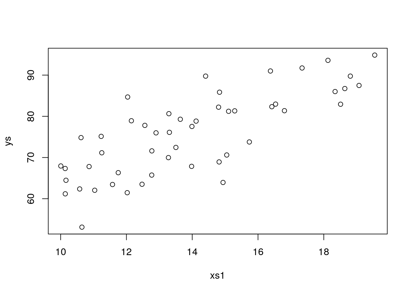
##
## Call:
## lm(formula = ys ~ xs1 + xs2 + xs3 + xs4)
##
## Residuals:
##      Min       1Q   Median       3Q      Max
## -10.3076  -2.7316   0.3072   2.2102   7.9088
##
## Coefficients:
##             Estimate Std. Error t value Pr(>|t|)
## (Intercept) 16.44303    7.42710   2.214   0.0319 *
## xs1          2.87327    0.21665  13.262  < 2e-16 ***
## xs2          1.93313    0.25274   7.649 1.12e-09 ***
## xs3         -0.47689    0.22325  -2.136   0.0381 *
## xs4         -0.08922    0.20937  -0.426   0.6720
## ---
## Signif. codes:  0 '***' 0.001 '**' 0.01 '*' 0.05 '.' 0.1 ' ' 1
##
## Residual standard error: 4.074 on 45 degrees of freedom
## Multiple R-squared:  0.8484,	Adjusted R-squared:  0.8349
## F-statistic: 62.94 on 4 and 45 DF,  p-value: < 2.2e-16
However, even after several runs, we never make a type II error. That must mean this setting has a large power, i.e. the ability to detect a true effect when one exists. Well, there are many ways to decrease power, like having a smaller sample size, increase the error or lower the true effect. Let’s try to increase the error, instead of the 4 used above, let’s pump it up10 fold to 40
seed<-100
set.seed(seed)
#define parameters
n<-50;b0<-5;b1<-3;b2<--2;error <- 40
#simulate potential explanatory variables
xs1=runif(n,10,20)
xs2=runif(n,10,20)
xs3=runif(n,10,20)
xs4=runif(n,10,20)
#simulate response
ys=b0+b1*xs1-b2*xs2+rnorm(n,sd=error)
#plot data
plot(xs1,ys)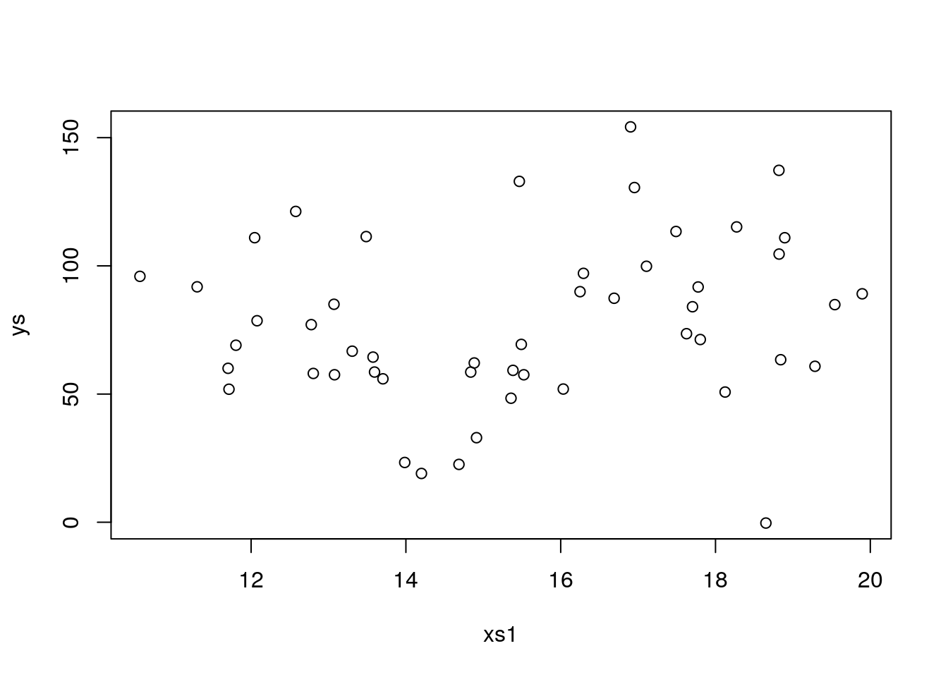
##
## Call:
## lm(formula = ys ~ xs1 + xs2 + xs3 + xs4)
##
## Residuals:
##    Min     1Q Median     3Q    Max
## -73.25 -17.86  -6.76  21.25  68.42
##
## Coefficients:
##             Estimate Std. Error t value Pr(>|t|)
## (Intercept)  22.8661    41.3133   0.553    0.583
## xs1           1.6034     1.8564   0.864    0.392
## xs2           0.9163     1.8092   0.506    0.615
## xs3           1.9650     1.6038   1.225    0.227
## xs4          -0.8544     1.7449  -0.490    0.627
##
## Residual standard error: 32.4 on 45 degrees of freedom
## Multiple R-squared:  0.06896,	Adjusted R-squared:  -0.0138
## F-statistic: 0.8333 on 4 and 45 DF,  p-value: 0.5112
That was an overkill, now there is so much noise must seeds we use do not allow us to find an effect, let’s cut that in half to 20
seed<-100
set.seed(seed)
#define parameters
n<-50;b0<-5;b1<-3;b2<--2;error <- 20
#simulate potential explanatory variables
xs1=runif(n,10,20)
xs2=runif(n,10,20)
xs3=runif(n,10,20)
xs4=runif(n,10,20)
#simulate response
ys=b0+b1*xs1-b2*xs2+rnorm(n,sd=error)
#plot data
plot(xs1,ys)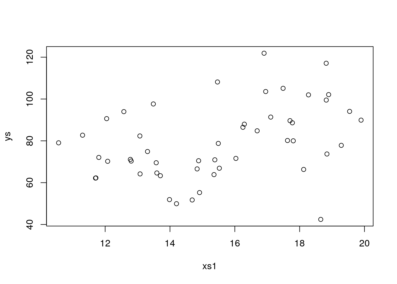
##
## Call:
## lm(formula = ys ~ xs1 + xs2 + xs3 + xs4)
##
## Residuals:
##     Min      1Q  Median      3Q     Max
## -36.624  -8.927  -3.380  10.623  34.211
##
## Coefficients:
##             Estimate Std. Error t value Pr(>|t|)
## (Intercept)  13.9330    20.6566   0.675    0.503
## xs1           2.3017     0.9282   2.480    0.017 *
## xs2           1.4582     0.9046   1.612    0.114
## xs3           0.9825     0.8019   1.225    0.227
## xs4          -0.4272     0.8724  -0.490    0.627
## ---
## Signif. codes:  0 '***' 0.001 '**' 0.01 '*' 0.05 '.' 0.1 ' ' 1
##
## Residual standard error: 16.2 on 45 degrees of freedom
## Multiple R-squared:  0.2262,	Adjusted R-squared:  0.1574
## F-statistic: 3.288 on 4 and 45 DF,  p-value: 0.01901
back to all correct. Now, let’s change seed again
seed<-103
set.seed(seed)
#define parameters
n<-50;b0<-5;b1<-3;b2<--2;error <- 20
#simulate potential explanatory variables
xs1=runif(n,10,20)
xs2=runif(n,10,20)
xs3=runif(n,10,20)
xs4=runif(n,10,20)
#simulate response
ys=b0+b1*xs1-b2*xs2+rnorm(n,sd=error)
#plot data
plot(xs1,ys)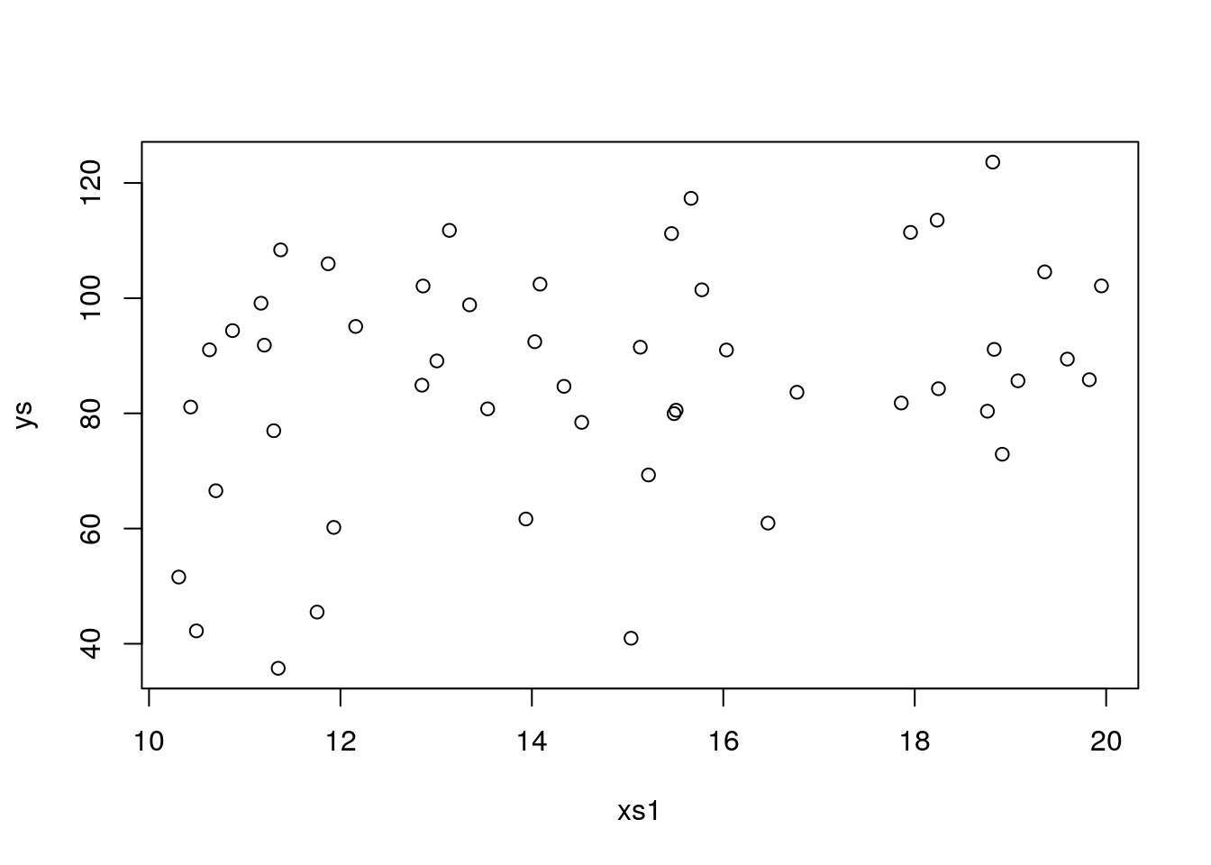
##
## Call:
## lm(formula = ys ~ xs1 + xs2 + xs3 + xs4)
##
## Residuals:
##     Min      1Q  Median      3Q     Max
## -36.079 -10.686  -0.148  16.413  33.845
##
## Coefficients:
##             Estimate Std. Error t value Pr(>|t|)
## (Intercept)  9.70575   33.83339   0.287   0.7755
## xs1          2.32559    0.93980   2.475   0.0172 *
## xs2          1.97688    1.20464   1.641   0.1078
## xs3          0.69013    1.02110   0.676   0.5026
## xs4          0.08031    0.97427   0.082   0.9347
## ---
## Signif. codes:  0 '***' 0.001 '**' 0.01 '*' 0.05 '.' 0.1 ' ' 1
##
## Residual standard error: 19.6 on 45 degrees of freedom
## Multiple R-squared:  0.1524,	Adjusted R-squared:  0.07706
## F-statistic: 2.023 on 4 and 45 DF,  p-value: 0.1073
Bang on, a type II error, as xs2 is no longer considered statistically significant. I am sure you can now play with the relevant model parameters, b1, b2, to incleare and decreese the actual effect, and with sample size n or as above with the error and explore the consequences of changing the balance in effect size, error and sample size on the ability of incurring in errors when doing regression. But remmeber the key, the reason we are able to see if an error is made or not is because we simulated reality. In this case, as it is never the case in an ecological dataset, we know the true model, which was
\[y=\beta_0+\beta_1 xs_1+\beta_2 xs2\]
That is the luxury of simulation, allowing you to test scenarios where “reality” is known, hence evaluating methods performance.
8.2 Task 2
The second task the students were faced was to create some regression data and the explore fitting models to it.
The data was simulated via this website: https://drawdata.xyz/ and was named data4lines.csv. Each student had its own dataset, here I work with my example.
We begin by reading the data in and plot it
#read the data
#folder<-"../Aula7 14 10 2020/"
folder<-"extfiles/"
data4lines <- read.csv(file=paste0(folder,"data4lines.csv"))
#plot all the data
plot(y~x,data=data4lines)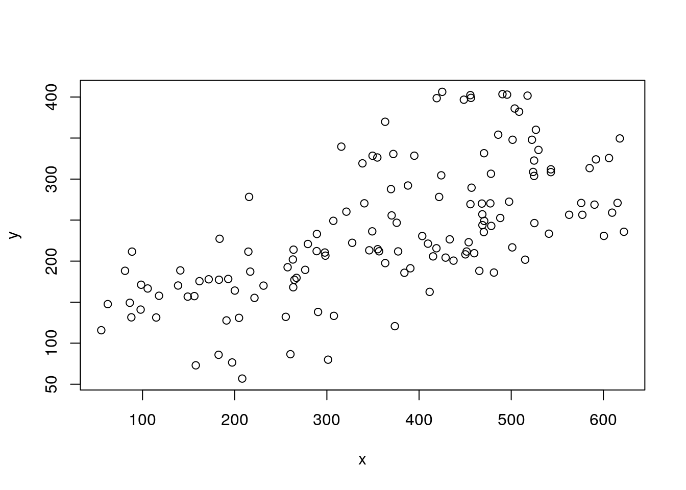
Now, to turn this a bit more interesting, we come up with a narrative.
These correspond to observations from weights and lenghts of a sample of animals, fish from the species Fishus inventadicus. We could fit a regression line to this data and see if we can predict weight from length
#plot all the data
plot(y~x,data=data4lines)
#fit model to pooled data
lmlinesG<-lm(y~x,data=data4lines)
abline(lmlinesG,lwd=3,lty=2)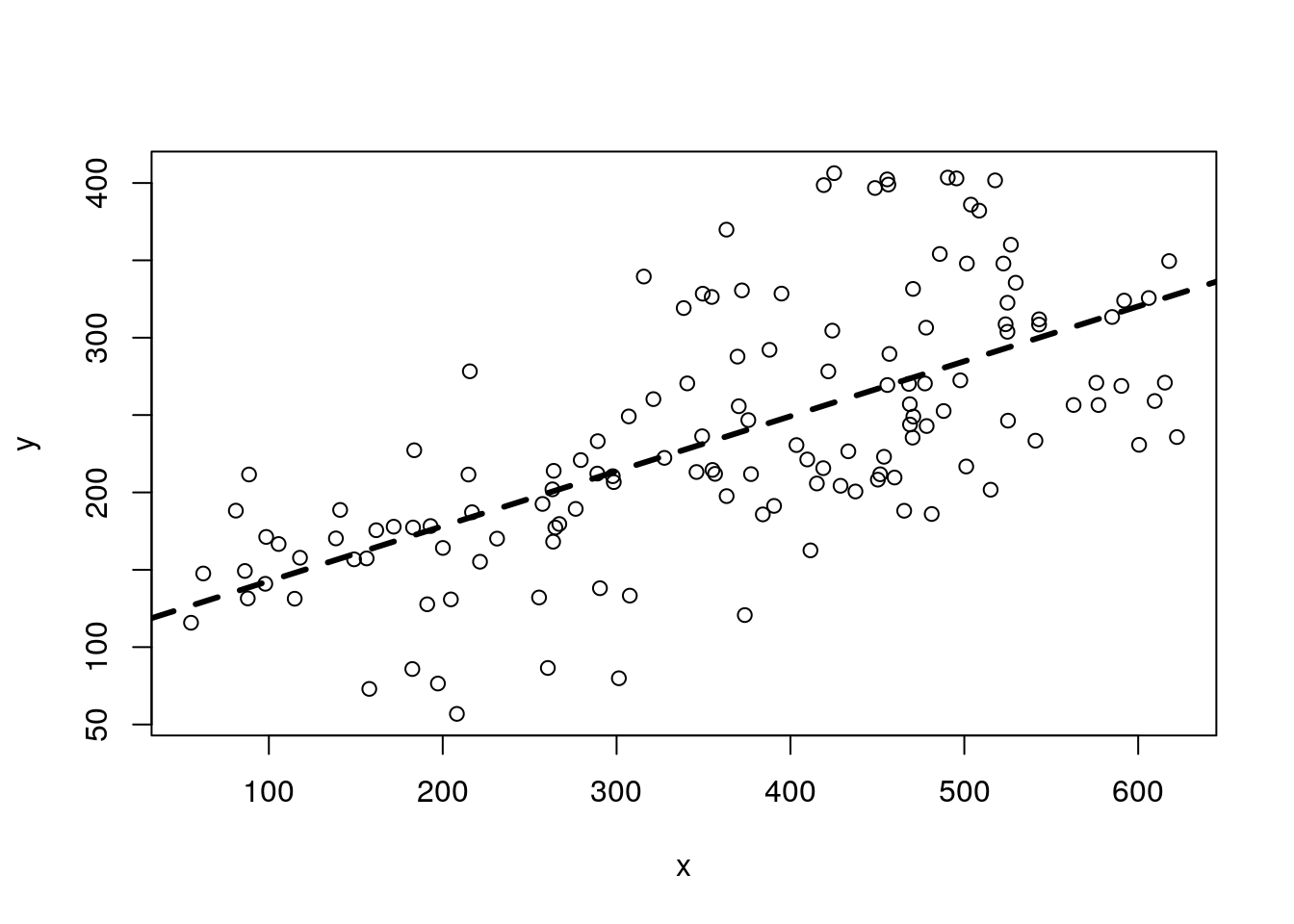
##
## Call:
## lm(formula = y ~ x, data = data4lines)
##
## Residuals:
##      Min       1Q   Median       3Q      Max
## -134.304  -44.188   -1.995   29.432  148.202
##
## Coefficients:
##              Estimate Std. Error t value Pr(>|t|)
## (Intercept) 107.17590   14.03069   7.639 3.51e-12 ***
## x             0.35513    0.03553   9.995  < 2e-16 ***
## ---
## Signif. codes:  0 '***' 0.001 '**' 0.01 '*' 0.05 '.' 0.1 ' ' 1
##
## Residual standard error: 61.78 on 136 degrees of freedom
## Multiple R-squared:  0.4235,	Adjusted R-squared:  0.4193
## F-statistic: 99.91 on 1 and 136 DF,  p-value: < 2.2e-16
and it looks like we can indeed predict the weight of the species from its length. The length is higly statistically significant. Not surprisingly, the longer the fish the heavier it is.
Now, the plot thickens. These animals actually came from 4 different museums, and are assumed to be the same species. However, a scientis decides to look at wether there are differences in the data from the 4 museums. So he colours the data by museum
#plot all the data
plot(y~x,col=as.numeric(as.factor(z)),data=data4lines,pch=1)
legend("topleft",inset=0.05,legend=letters[1:4],col=1:4,pch=1)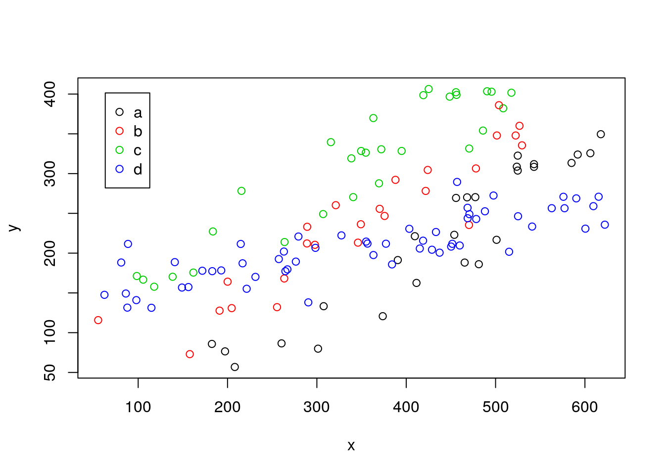
We see a patter in the data, the data from the different museums tend to cluster. He decides to investigate. Note folks providing names to museum in this country are a bit borring, and the museums are called “a”, “b”, “c” and “d”.
Our smart researcher says: “well, it seems like the relationship might be different in each museum”. Then, maybe I should fit a model that includes museum as a covariate weight~length+museum.
\[y=\beta_0+\beta_1 \times length +\beta_2 \times museum\]
And so he does and plots it
##
## Call:
## lm(formula = y ~ x + z, data = data4lines)
##
## Residuals:
##    Min     1Q Median     3Q    Max
## -90.01 -35.01   2.54  35.51 108.10
##
## Coefficients:
##              Estimate Std. Error t value Pr(>|t|)
## (Intercept)  45.51813   13.83069   3.291  0.00128 **
## x             0.39657    0.02516  15.763  < 2e-16 ***
## zb           54.92376   12.11597   4.533 1.28e-05 ***
## zc          128.20339   11.72572  10.934  < 2e-16 ***
## zd           22.82412   10.26509   2.223  0.02787 *
## ---
## Signif. codes:  0 '***' 0.001 '**' 0.01 '*' 0.05 '.' 0.1 ' ' 1
##
## Residual standard error: 42.5 on 133 degrees of freedom
## Multiple R-squared:  0.7332,	Adjusted R-squared:  0.7252
## F-statistic: 91.38 on 4 and 133 DF,  p-value: < 2.2e-16
The output shows that the length is relevant, but the museum is relevant too. The relationship might be different per museum! In the output we see the x, the length, but not the z, it has been transformed into zb, zc and zd. Why is that? That is a mistery that we shall unfold now!
While the model we are fitting might be represented by weight~length+museum, th edesign matrix being fitted replaces the museum (a factor with 4 levels) with 3 dummy variables (a factor with k levels required k-1 dummy variables). So the real model being fitted is really
\[y=\beta_0+\beta_1 \times length + \beta_{2b} \times zb + \beta_{2c} \times zc + \beta_{2d} \times zd\]
Wait, but where is the level a? It is in the intercept, and if I had an euro for each time that confused a student, I would not be here but in a beach in the Bahamas having a piña colada :)
But let’s unfold the mistery, shall we? By default, R takes 1 level of (each/a) factor and uses it as the intercept. Here it used a (the choice is in this case by alphabetical ored, but one can change that, which might be useful if e.g. you want to have as the intercept a control level, say; look e.g. into function factor help to see how you can change the baseline level of a factor).
Hence, the intercept for museum a is 45.5181335. What about the intercep of the othe rmuseums? They are always reported with a as the reference. Look at the equation above, what happens when say zc is 1 and zd and zb are 0, it becomes
\[y=\beta_0+\beta_1 \times length + \beta_{2c} \times zc \] \[y=(\beta_0+\beta_{2c})+\beta_1 \times length = intercep + slope \times length\]
and so, from the above output, that equates to y=lmlines$coefficients[1]+lmlines$coefficients[4],lmlines$coefficients[2] or 173.7215247+0.3965715 \(\times\) length.
So now we can add all these estimated regression lines to the plot
#plot all
plot(y~x,col=z,data=data4lines)
legend("topleft",inset=0.05,legend=c(LETTERS[1:4],"all"),col=c(1:4,1),lty=c(rep(1,4),2),lwd=c(rep(1,4),3))
#these are the wrong lines... why?
abline(lmlinesG,lwd=3,lty=2)
abline(lmlines$coefficients[1],lmlines$coefficients[2],col=1)
abline(lmlines$coefficients[1]+lmlines$coefficients[3],lmlines$coefficients[2],col=2)
abline(lmlines$coefficients[1]+lmlines$coefficients[4],lmlines$coefficients[2],col=3)
abline(lmlines$coefficients[1]+lmlines$coefficients[5],lmlines$coefficients[2],col=4)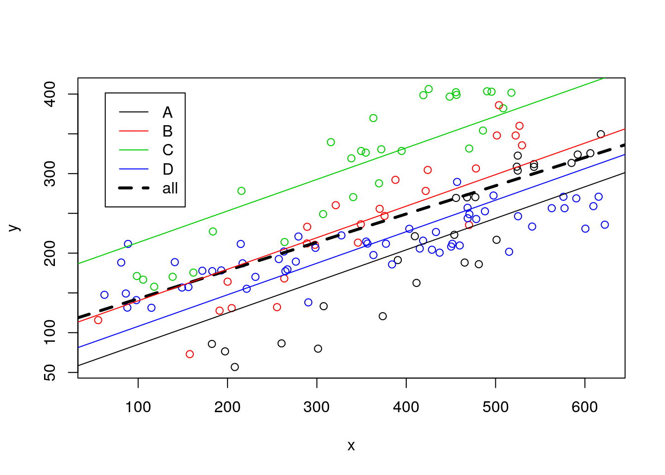
note that, not surprisingly, all these lines have the same slope. Or in other words, the model we considered assumes that the slope of the model is the same across museums (which, remember, we know if not true!). We can easily check that the intercepts (i.e. where the lines cross when length=x=0) of all lines are indeed easy to get from the model’s output
#plot all
plot(y~x,xlim=c(-10,700),ylim=c(0,450),col=z,data=data4lines)
legend("topleft",inset=0.05,legend=c(LETTERS[1:4],"all"),col=c(1:4,1),lty=c(rep(1,4),2),lwd=c(rep(1,4),3))
#these are the wrong lines... why?
abline(lmlinesG,lwd=3,lty=2)
abline(lmlines$coefficients[1],lmlines$coefficients[2],col=1)
abline(lmlines$coefficients[1]+lmlines$coefficients[3],lmlines$coefficients[2],col=2)
abline(lmlines$coefficients[1]+lmlines$coefficients[4],lmlines$coefficients[2],col=3)
abline(lmlines$coefficients[1]+lmlines$coefficients[5],lmlines$coefficients[2],col=4)


abline(v=0,lty=2)
abline(h=45.51813,lty=2,col=1)
abline(h=45.51813+54.92376,lty=2,col=2)
abline(h=45.51813+128.20339,lty=2,col=3)
abline(h=45.51813+22.82412,lty=2,col=4)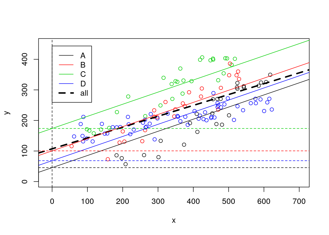
Now, the smart biologist then says that he could also fit a separate line to each museum’s data. And so he does, and that looks like this:
#plot all the data
plot(y~x,col=as.numeric(as.factor(z)),data=data4lines,pch=1)
#completely independet regression lines
abline(lm(y~x,data=data4lines[data4lines$z=="a",]),col=1,lty=4)
abline(lm(y~x,data=data4lines[data4lines$z=="b",]),col=2,lty=4)
abline(lm(y~x,data=data4lines[data4lines$z=="c",]),col=3,lty=4)
abline(lm(y~x,data=data4lines[data4lines$z=="d",]),col=4,lty=4)
legend("topleft",inset=0.05,legend=letters[1:4],col=1:4,pch=1)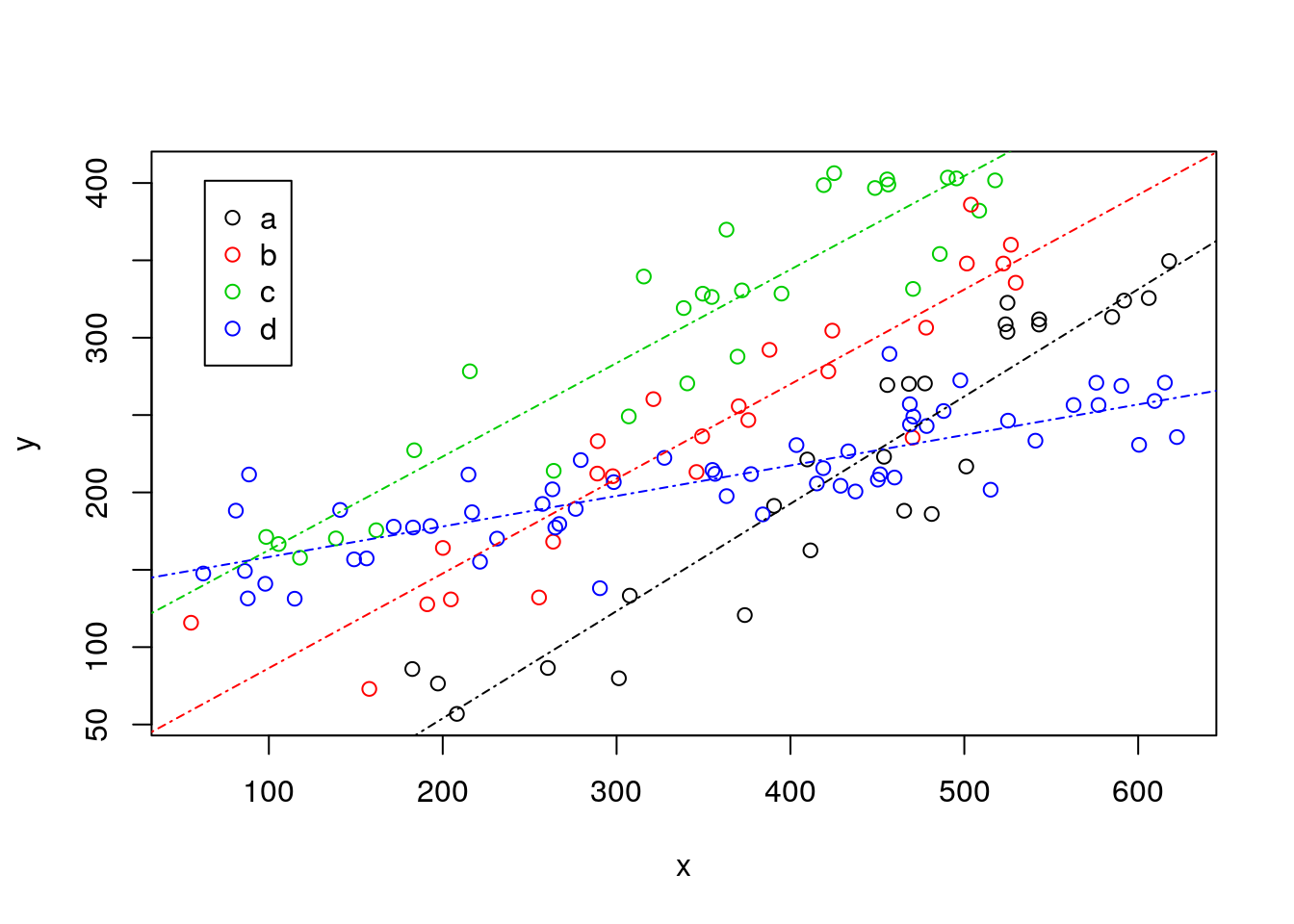
Naturally, now the lines do not have the same slope, and we can compare all these in a single plot. This plot is really messy, as it includes the pooled regression (the thick black line), the regressions fitted to independent data sets, one for each museum (the solid lines), and the regressions resulting from the model with museum as a factor covariate (dotted-dashed lines).
#plot all the data
plot(y~x,col=as.numeric(as.factor(z)),data=data4lines,pch=1)
#completely independet regression lines
abline(lm(y~x,data=data4lines[data4lines$z=="a",]),col=1,lty=4)
abline(lm(y~x,data=data4lines[data4lines$z=="b",]),col=2,lty=4)
abline(lm(y~x,data=data4lines[data4lines$z=="c",]),col=3,lty=4)
abline(lm(y~x,data=data4lines[data4lines$z=="d",]),col=4,lty=4)
#these are the wrong lines... why?
abline(lmlinesG,lwd=3,lty=2)
abline(lmlines$coefficients[1],lmlines$coefficients[2],col=1)
abline(lmlines$coefficients[1]+lmlines$coefficients[3],lmlines$coefficients[2],col=2)
abline(lmlines$coefficients[1]+lmlines$coefficients[4],lmlines$coefficients[2],col=3)
abline(lmlines$coefficients[1]+lmlines$coefficients[5],lmlines$coefficients[2],col=4)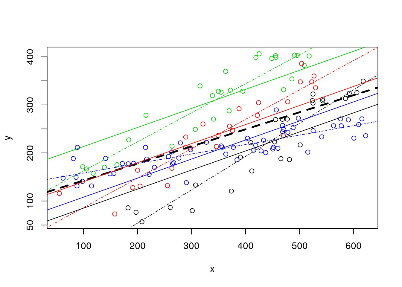
But what is the best model to describe the data? That is a mistery that will remain to unfold. For that we will need and additional complication in a regression model: interactions.
But note 1 thing to begin with. The pooled model uses just 2 parameters, one slope and one intercept. The independent lines use 8 parameters, 4 slopes and 4 intercepts, one line for each museum. And the single model with lenght and museum uses 5 parameters, the intercept, the slope for length, and 3 parameters associated with the \(k-1=3\) levels of museum (remember, one level of each factor is absorbed by the regression intercept).
So the choice of what is best might be not straightforward. While we created the data by hand, we do not know the true model! Choosing the best model requires choosing between models with different complexity, i.e. different number of parameters. We will need a parsimonious model, one that describes the data well, but with a number of parameters that is not too high for the available data. That will also require selection criteria.
Stay tuned for the next episodes on our regression saga!