5 Predicting 2018-19 Season Results From Prior Data
Our next goal of this research project is to look at different models of predicting the outcome of a Premier League season. Additionally, we would like to compare models based on different sets of data. Here we’re going to predict the 2018-19 season results using 3 different subset of years: 1) using data from all seasons prior to 2018-19, 2) from only the 2010s, 3) from all seasons, but with different weights on the seasons, with more weight being put toward more recent competitions.
5.1 Using Data From Every Year Before 2018-19
5.1.1 Data Transforming
We first get a new data frame with matches from last year being filtered out, since we want to use data prior to 2018-19 to predict the results of last season.
For later purposes, we’re going to go ahead and grab the team names from the table, and created a data frame called “Teams.”
Teams <- as.data.frame(unique(epl.data$HomeTeam))
colnames(Teams) <- c("TeamName")
Teams <- arrange(Teams, TeamName)
We now create Poisson regression models and use them to get the scoring rates for all teams at home and on the road. Poisson Regression is a member of a broad class of models known as the Generalized Linear Models (GLM). A generalized linear model has the general form
\[\displaystyle E(Y_i) = \mu_i = g^{-1}(\beta_0 + \beta_1 X_{i1} + \beta_2 X_{i2} + \ldots + \beta_k X_{ik})\]
There are three main components to a generalized linear model:
A random component, indicating the conditional distribution of the response variable \(Y_i\) (for the \(i\)th of \(n\) independently sampled observations), given the values of the explanatory variables. \(Y_i\)’s distribution must be a member of an exponential family, such as Gaussian, Binomial, Poisson, or Gamma.
A linear predictor (\(\beta_0 + \beta_1 X_1 + \beta_2 X_2 + \ldots + \beta_k X_k\)), which is a linear combination of the explanatory variables (the \(X\)’s), with the \(\beta\)’s as the regression coefficients to be estimated.
A canonical link function \(g\), which transforms the expected value of the response variable, \(E(Y_i) = \mu_i\), to the linear predictor.
Poisson regression models are generalized linear models with the logarithm as the link function. It is used when our response’s data type is a count, which is appropriate for our case since our count variable is the number of goals scored. The model assumes that observed outcome variable follows a Poisson distribution and attempts to fit the mean parameter to a linear model of explanatory variables.
The regression equation for a Poisson regression model is of the form
\[\displaystyle \mu_i = e^{\ \beta_0 + \beta_1 X_{i1} + \beta_2 X_{i2} + \ldots + \beta_k X_{ik}}\] or equivalently,
\[\displaystyle ln(\mu_i) = \beta_0 + \beta_1 X_{i1} + \beta_2 X_{i2} + \ldots + \beta_k X_{ik}\]
We first do Poisson regression to get every team’s scoring rate when playing at home.
Our next step is to get the regression coefficients (all the \(\beta\)’s) for every team from this model, alongside with the model’s y-intercept, which will allow us to make predictions later on. For this reason, we’re going to create a data frame with all coefficients from the model. Since we want a table of every team’s coefficient, and the first row of our current coefficients table contains the y-intercept of our regression model, we’re going to replace it by 0, which is the coefficient for the reference team. By default, R uses the team that comes first alphabetically to be the reference group, which is Arsenal.
# get the coefficients
HomeTable <- as.data.frame(coefficients(HomeReg))
names(HomeTable)[1] <- "Coeff"
HomeIntercept <- HomeTable[1,1] # get the model's y-intercept
HomeTable[1,1] <- 0 # reference group
HomeTable[,2] <- Teams$TeamName # put the team names into table
names(HomeTable)[2] <- "HomeTeam"
We can now use our Poisson Regression model to make predictions by evaluating the model equation at different values of the explanatory variable. We, however, first must back-transform the equation to a meaningful scale. Since the link function for Poisson regression is the natural log (ln) function, we’d back-transform with the corresponding exponential function.
##         (Intercept) HomeTeamAston Villa    HomeTeamBarnsley
##           0.7131765          -0.4451672          -0.4387396
Here, we’re going to back transform in order to predict the mean (expected) home scoring rate for every team. For example, Aston Villa has a coefficient value of -0.445, and to get the mean goal scoring rate for this team (aggregated across all opponents), we take \(e\) raised to (intercept + coefficient) power, which equals to \(e^{0.713 - 0.445}\) = 1.307 goals/match.
HomeTable <- HomeTable %>%
  mutate(HomeRate = round(exp(HomeIntercept + Coeff), 3),
         FakeCol = "fake") # fake column for joining purpose
Below is a look at our table with all the Premier League teams and their home scoring rates.
| Coeff | HomeTeam | HomeRate |
|---|---|---|
| 0.0000000 | Arsenal | 2.040 |
| -0.4451672 | Aston Villa | 1.307 |
| -0.4387396 | Barnsley | 1.316 |
| -0.5159293 | Birmingham | 1.218 |
We are now going to do this process again to get team’s away scoring rates.
AwayReg <- glm(Away.Goals ~ AwayTeam,
            family = poisson(link = "log"),
            data = epl.data)
AwayTable <- as.data.frame(coefficients(AwayReg))
names(AwayTable)[1] <- "Coeff"
AwayIntercept <- AwayTable[1,1]
AwayTable[1,1] <- 0
AwayTable[,2] <- Teams$TeamName
names(AwayTable)[2] <- "AwayTeam"
AwayTable <- AwayTable %>%
  mutate(AwayRate = round(exp(AwayIntercept + Coeff), 3),
         FakeCol = "fake")
We then use a full join to join the 2 tables together into a big data frame consisting all the possible matchups with teams’ home and away rates.
FullTable <- full_join(HomeTable, AwayTable, by = "FakeCol")
FullTable <- FullTable %>%
  filter(HomeTeam != AwayTeam) %>%
  select(HomeTeam, HomeRate, AwayTeam, AwayRate)
We now have a table of all possible matchups and all the home and away rates. Our job now is to remove teams that did not participate last year from our table.
Teams1819 <- epl.fulldata %>%   # get the 18-19 teams
  filter(Season == "2018-2019") %>%
  select(HomeTeam)
Teams1819 <- unique(Teams1819)

Table1819 <- FullTable %>%   # only keep 18-19 teams
  filter(HomeTeam %in% Teams1819$HomeTeam,
AwayTeam %in% Teams1819$HomeTeam)## [1] 380Here’s a quick glimpse at our table. It has 380 rows, representing the 380 total team matchups of the season. In each Premier League season a club gets to play every other squad twice, once on their home pitch and once on the other team’s field. As we can see from our table below, the first matchup is Arsenal - Bournemouth, at Arsenal. There is also a row for a game between these two teams, but in reverse order, with Bournemouth playing at home against Arsenal.
| HomeTeam | HomeRate | AwayTeam | AwayRate |
|---|---|---|---|
| Arsenal | 2.04 | Bournemouth | 1.145 |
| Arsenal | 2.04 | Brighton | 0.684 |
| Arsenal | 2.04 | Burnley | 0.895 |
We are now set to simulate!
5.1.2 Simulation
We would like to simulate the results of the 2018-19 seasons 10000 times. Our goal is to get the team’s ranking, their total points, and their goal differential for each simulated season. Our current table Table1819 currently has 380 rows representing all possible matchups of the 2018-19 seasons. To create of 10000 simulations, we duplicate this table 10000 times, and create a new table called SimTable.
nSim <- 10000  # duplicate the 2018-19 table 10000 times
SimTable <- Table1819 %>%
  slice(rep(row_number(), nSim)) # rep(): replicate the rows
                                 # slice(): choose rows
We then use the rpois function to generate the number of goals scored for every home and away team in every row of our table. In addition, the number of points for every match outcome based on the teams’ number of goals scored are also calculated, as a side gets 3 points if it scores more than its opponent, 1 point if it’s a tie, and 0 points if the opposing roster has more goals.
SimTable <- SimTable %>%
  mutate(HomeScore = rpois(nrow(SimTable), HomeRate),
         AwayScore = rpois(nrow(SimTable), AwayRate),
         HomePoints = ifelse(HomeScore > AwayScore, 3,
                             ifelse(HomeScore == AwayScore, 1, 0)),
         AwayPoints = ifelse(HomeScore > AwayScore, 0,
                             ifelse(HomeScore == AwayScore, 1, 3)))
Here’s a look at the current version of our SimTable. The two columns HomeScore and AwayScore indicate our simulate match outcome for each matchup, as they are the number of goals scored for each club randomly generated using their scoring rates. To get these goal values, we use the rpois function in R, which takes in the scoring rate for each team and returns a random integer for number of goals scored. For example, in the third row of the table below, Arsenal, on their home pitch, defeats Burnley by 4 goals to 2. Arsenal, hence, earns a valuable 3 points for winning the match; Burnley, on the other hand, gets no points for their loss.
| HomeTeam | HomeRate | AwayTeam | AwayRate | HomeScore | AwayScore | HomePoints | AwayPoints |
|---|---|---|---|---|---|---|---|
| Arsenal | 2.040462 | Bournemouth | 1.1447368 | 1 | 0 | 3 | 0 |
| Arsenal | 2.040462 | Brighton | 0.6842105 | 1 | 1 | 1 | 1 |
| Arsenal | 2.040462 | Burnley | 0.8947368 | 4 | 2 | 3 | 0 |
| Arsenal | 2.040462 | Cardiff | 0.6578947 | 3 | 2 | 3 | 0 |
## [1] 3800000Since each season has 380 games and we duplicated the table 10000 times, the SimTable has a total of 3800000 rows. We can say that every 380-row segment contains the result of 1 simulated season. We then write this function to get each individual simulation and also tally up the points, calculate goal differentials and get the team ranking for each season.
Sim <- function(simNum){
  firstRow <- 380*simNum - 379 # first row of each season
  lastRow <- 380*simNum        # last row
  MyTable <- SimTable[firstRow:lastRow,] # get each season's table

  Home1819 <- MyTable %>%      # get home results
    group_by(HomeTeam) %>%
    summarise(TotalHomePoints = sum(HomePoints), # points
              TotalHomeScored = sum(HomeScore),  # goals scored
              TotalHomeConceded = sum(AwayScore)) %>% # goals conceded
    rename(Team = HomeTeam)

  Away1819 <- MyTable %>%      # get away results
    group_by(AwayTeam) %>%
    summarise(TotalAwayPoints = sum(AwayPoints),
              TotalAwayScored = sum(AwayScore),
              TotalAwayConceded = sum(HomeScore)) %>%
    rename(Team = AwayTeam)

  # join home and away tables
  PointsTable <- full_join(Home1819, Away1819)

  # calculate total points and GD (= goals scored - conceded)
  PointsTable <- PointsTable %>%
    mutate(FinalPoints = TotalHomePoints + TotalAwayPoints,
           GD = TotalHomeScored - TotalHomeConceded +
                TotalAwayScored - TotalAwayConceded) %>%
    arrange(desc(FinalPoints), desc(GD)) %>%
    mutate(SimNum = simNum, # distinguish the sim's
           Rank = 1:20) %>% # rank for each team
    select(Rank, Team, FinalPoints, GD, SimNum)
}
Here are 2 sample simulated seasons we got by using this function.
| Rank | Team | FinalPoints | GD | SimNum |
|---|---|---|---|---|
| 1 | Arsenal | 79 | 36 | 1 |
| 2 | Liverpool | 72 | 24 | 1 |
| 3 | Chelsea | 72 | 21 | 1 |
| 4 | Man United | 65 | 16 | 1 |
| 5 | Brighton | 64 | 3 | 1 |
| 6 | Man City | 57 | 9 | 1 |
| 7 | West Ham | 56 | 1 | 1 |
| 8 | Tottenham | 55 | 6 | 1 |
| 9 | Newcastle | 55 | 0 | 1 |
| 10 | Crystal Palace | 51 | 0 | 1 |
| 11 | Watford | 50 | -5 | 1 |
| 12 | Fulham | 49 | 0 | 1 |
| 13 | Southampton | 47 | 2 | 1 |
| 14 | Leicester | 44 | -1 | 1 |
| 15 | Everton | 43 | -18 | 1 |
| 16 | Burnley | 41 | -13 | 1 |
| 17 | Bournemouth | 40 | -12 | 1 |
| 18 | Wolves | 39 | -19 | 1 |
| 19 | Huddersfield | 38 | -20 | 1 |
| 20 | Cardiff | 27 | -30 | 1 |
| Rank | Team | FinalPoints | GD | SimNum |
|---|---|---|---|---|
| 1 | Man United | 69 | 21 | 2 |
| 2 | Liverpool | 68 | 18 | 2 |
| 3 | Chelsea | 67 | 19 | 2 |
| 4 | Arsenal | 66 | 20 | 2 |
| 5 | Man City | 63 | 15 | 2 |
| 6 | Bournemouth | 60 | 11 | 2 |
| 7 | West Ham | 56 | 2 | 2 |
| 8 | Leicester | 55 | 4 | 2 |
| 9 | Southampton | 54 | 1 | 2 |
| 10 | Wolves | 53 | -10 | 2 |
| 11 | Newcastle | 50 | 3 | 2 |
| 12 | Crystal Palace | 49 | -7 | 2 |
| 13 | Brighton | 48 | -10 | 2 |
| 14 | Tottenham | 45 | -12 | 2 |
| 15 | Watford | 44 | -12 | 2 |
| 16 | Fulham | 43 | -8 | 2 |
| 17 | Everton | 42 | -7 | 2 |
| 18 | Burnley | 42 | -11 | 2 |
| 19 | Cardiff | 37 | -20 | 2 |
| 20 | Huddersfield | 32 | -17 | 2 |
Now we’re interested in getting the result of each one of our 10000 simulations and put everything together into a data frame. We utilize a for loop to get every simulation and a full_join to combine our simulations into a big table called EPLSim_All.
5.1.3 Analysis
After the simulation is complete, we write the simulation table to a csv file and name it EPLSimFull.csv. We can now import the data file and do some analysis.
EPLSim_All <- read.csv("EPLSimFull.csv")
EPLSim_All <- EPLSim_All %>%
  mutate(SimType = "All Seasons")
5.1.3.1 Team Rankings
We now obtain a table of every 2018-19 team’s chance of finishing at each position on the final standing table from our simulation, as shown by the below ouput table.
AllRankTable <- table(EPLSim_All$Team, EPLSim_All$Rank)/nSim
AllRankTable %>%
  mykable() %>%
scroll_box(width = "100%")| 1 | 2 | 3 | 4 | 5 | 6 | 7 | 8 | 9 | 10 | 11 | 12 | 13 | 14 | 15 | 16 | 17 | 18 | 19 | 20 | |
|---|---|---|---|---|---|---|---|---|---|---|---|---|---|---|---|---|---|---|---|---|
| Arsenal | 0.1968 | 0.1850 | 0.1542 | 0.1215 | 0.0953 | 0.0745 | 0.0519 | 0.0384 | 0.0259 | 0.0179 | 0.0126 | 0.0092 | 0.0052 | 0.0046 | 0.0035 | 0.0017 | 0.0008 | 0.0009 | 0.0001 | 0.0000 |
| Bournemouth | 0.0077 | 0.0175 | 0.0312 | 0.0462 | 0.0562 | 0.0672 | 0.0743 | 0.0816 | 0.0858 | 0.0839 | 0.0856 | 0.0715 | 0.0652 | 0.0548 | 0.0493 | 0.0424 | 0.0320 | 0.0253 | 0.0157 | 0.0066 |
| Brighton | 0.0000 | 0.0002 | 0.0008 | 0.0012 | 0.0036 | 0.0040 | 0.0086 | 0.0116 | 0.0163 | 0.0270 | 0.0355 | 0.0447 | 0.0557 | 0.0707 | 0.0844 | 0.0994 | 0.1198 | 0.1341 | 0.1499 | 0.1325 |
| Burnley | 0.0002 | 0.0006 | 0.0021 | 0.0044 | 0.0072 | 0.0112 | 0.0163 | 0.0213 | 0.0319 | 0.0378 | 0.0441 | 0.0565 | 0.0723 | 0.0776 | 0.0883 | 0.1015 | 0.1107 | 0.1154 | 0.1100 | 0.0906 |
| Cardiff | 0.0001 | 0.0000 | 0.0008 | 0.0014 | 0.0019 | 0.0028 | 0.0052 | 0.0079 | 0.0131 | 0.0170 | 0.0267 | 0.0319 | 0.0467 | 0.0552 | 0.0754 | 0.0953 | 0.1187 | 0.1444 | 0.1670 | 0.1885 |
| Chelsea | 0.1428 | 0.1560 | 0.1520 | 0.1298 | 0.1056 | 0.0822 | 0.0613 | 0.0490 | 0.0357 | 0.0250 | 0.0186 | 0.0137 | 0.0108 | 0.0067 | 0.0045 | 0.0032 | 0.0016 | 0.0009 | 0.0004 | 0.0002 |
| Crystal Palace | 0.0011 | 0.0039 | 0.0078 | 0.0119 | 0.0196 | 0.0255 | 0.0340 | 0.0420 | 0.0521 | 0.0600 | 0.0708 | 0.0741 | 0.0832 | 0.0846 | 0.0848 | 0.0884 | 0.0808 | 0.0730 | 0.0612 | 0.0412 |
| Everton | 0.0100 | 0.0245 | 0.0378 | 0.0539 | 0.0630 | 0.0692 | 0.0769 | 0.0844 | 0.0882 | 0.0829 | 0.0737 | 0.0668 | 0.0638 | 0.0583 | 0.0466 | 0.0376 | 0.0276 | 0.0174 | 0.0118 | 0.0056 |
| Fulham | 0.0018 | 0.0067 | 0.0115 | 0.0189 | 0.0300 | 0.0427 | 0.0522 | 0.0600 | 0.0674 | 0.0750 | 0.0861 | 0.0855 | 0.0831 | 0.0757 | 0.0799 | 0.0647 | 0.0601 | 0.0477 | 0.0347 | 0.0163 |
| Huddersfield | 0.0001 | 0.0001 | 0.0000 | 0.0004 | 0.0005 | 0.0009 | 0.0021 | 0.0025 | 0.0040 | 0.0086 | 0.0120 | 0.0161 | 0.0247 | 0.0353 | 0.0475 | 0.0651 | 0.0886 | 0.1325 | 0.2003 | 0.3587 |
| Leicester | 0.0066 | 0.0160 | 0.0266 | 0.0372 | 0.0500 | 0.0601 | 0.0741 | 0.0756 | 0.0826 | 0.0834 | 0.0820 | 0.0811 | 0.0705 | 0.0632 | 0.0544 | 0.0433 | 0.0380 | 0.0254 | 0.0214 | 0.0085 |
| Liverpool | 0.1250 | 0.1494 | 0.1398 | 0.1321 | 0.1102 | 0.0835 | 0.0685 | 0.0545 | 0.0371 | 0.0319 | 0.0215 | 0.0159 | 0.0112 | 0.0077 | 0.0059 | 0.0026 | 0.0022 | 0.0005 | 0.0005 | 0.0000 |
| Man City | 0.0700 | 0.1063 | 0.1208 | 0.1106 | 0.1093 | 0.1041 | 0.0836 | 0.0707 | 0.0584 | 0.0455 | 0.0353 | 0.0248 | 0.0198 | 0.0145 | 0.0116 | 0.0075 | 0.0034 | 0.0024 | 0.0012 | 0.0002 |
| Man United | 0.3699 | 0.2114 | 0.1375 | 0.0919 | 0.0617 | 0.0447 | 0.0274 | 0.0180 | 0.0134 | 0.0081 | 0.0070 | 0.0040 | 0.0017 | 0.0017 | 0.0009 | 0.0005 | 0.0001 | 0.0001 | 0.0000 | 0.0000 |
| Newcastle | 0.0180 | 0.0347 | 0.0450 | 0.0679 | 0.0815 | 0.0876 | 0.0892 | 0.0906 | 0.0839 | 0.0770 | 0.0651 | 0.0608 | 0.0528 | 0.0430 | 0.0350 | 0.0265 | 0.0174 | 0.0131 | 0.0077 | 0.0032 |
| Southampton | 0.0053 | 0.0123 | 0.0214 | 0.0311 | 0.0447 | 0.0574 | 0.0664 | 0.0713 | 0.0774 | 0.0796 | 0.0822 | 0.0790 | 0.0736 | 0.0729 | 0.0610 | 0.0571 | 0.0424 | 0.0330 | 0.0220 | 0.0099 |
| Tottenham | 0.0391 | 0.0637 | 0.0866 | 0.0999 | 0.1029 | 0.1003 | 0.0998 | 0.0817 | 0.0696 | 0.0608 | 0.0480 | 0.0446 | 0.0305 | 0.0258 | 0.0185 | 0.0106 | 0.0074 | 0.0053 | 0.0038 | 0.0011 |
| Watford | 0.0002 | 0.0009 | 0.0026 | 0.0057 | 0.0095 | 0.0132 | 0.0186 | 0.0303 | 0.0336 | 0.0425 | 0.0527 | 0.0656 | 0.0732 | 0.0880 | 0.0914 | 0.0991 | 0.1101 | 0.1038 | 0.0907 | 0.0683 |
| West Ham | 0.0047 | 0.0090 | 0.0164 | 0.0261 | 0.0362 | 0.0480 | 0.0640 | 0.0726 | 0.0784 | 0.0862 | 0.0794 | 0.0826 | 0.0796 | 0.0731 | 0.0651 | 0.0574 | 0.0466 | 0.0380 | 0.0226 | 0.0140 |
| Wolves | 0.0006 | 0.0018 | 0.0051 | 0.0079 | 0.0111 | 0.0209 | 0.0256 | 0.0360 | 0.0452 | 0.0499 | 0.0611 | 0.0716 | 0.0764 | 0.0866 | 0.0920 | 0.0961 | 0.0917 | 0.0868 | 0.0790 | 0.0546 |
For example, if we look at row 1, Arsenal has a 0.1968 (19.68%) probability of finishing first, 18.5% chance of finishing second, and so on and so forth. To get the probability of Arsenal finishing at least at a certain position, we can just simply add up the probabilities of being at or above that position. For example, Arsenal’s chance of finishing in the top 4 is the sum of their probabilities of ending at position 1, 2, 3, and 4, which is 0.1968 + 0.1850 + 0.1542 + 0.1215 = 0.6575 = 65.75%.
We want to look at some specific categories of team rankings, so now we’re going to examine the following notable places of the league table: first place, top 4, and bottom 3.
5.1.3.2 First Place
EPLSim_All %>%
  filter(Rank == 1) %>%
  group_by(Team) %>%
  summarise(Pct = 100*n()/(nSim)) %>%
  arrange(desc(Pct)) %>%
  head(6) %>%
mykable()| Team | Pct |
|---|---|
| Man United | 36.99 |
| Arsenal | 19.68 |
| Chelsea | 14.28 |
| Liverpool | 12.50 |
| Man City | 7.00 |
| Tottenham | 3.91 |
Just like many top sports leagues around the world, the team that finishes first at the end of each Premier League season will be crowned league champions and will get to take the trophy home with them. The table above shows the 6 teams with the highest chance of winning the 2018-19 season based on our simulation results. Unsurprisingly, they are the infamous Premier League’s “Big 6” - Manchester United, Arsenal, Chelsea, Liverpool, Manchester City and Tottenham. Man Utd leads the way by winning 36.99% of the seasons, or 3699 out of 10000 simulated seasons; followed by Arsenal, Chelsea, and so on. Since we’re using data from all Premier League seasons and Man Utd is the winningest club in the history of top tier English football, in terms of both number of titles and matches, it completely makes sense why they won the title race more than any other club in our simulations.
5.1.3.3 Top 4
EPLSim_All %>%
  filter(Rank %in% c(1,2,3,4)) %>%
  group_by(Team) %>%
  summarise(Pct = 100*n()/(nSim)) %>%
  arrange(desc(Pct)) %>%
  head(6) %>%
mykable()| Team | Pct |
|---|---|
| Man United | 81.07 |
| Arsenal | 65.75 |
| Chelsea | 58.06 |
| Liverpool | 54.63 |
| Man City | 40.77 |
| Tottenham | 28.93 |
The significance for a ball club to finish in the top 4 of the Premier League is that they would punch their tickets to the UEFA Champions League, an annual competition contested by top football clubs in Europe. Based on the table above, the big 6 once again dominate this category, as Manchester United has the highest chance making the top 4 at 81.07. Arsenal, Chelsea and Liverpool each secures a Champions League spot in more than half of the 10000 simulations. In reality, the 4 teams that claimed the top 4 spots of the table last year in order were Man City, Liverpool, Chelsea, and Tottenham; followed by Arsenal at fifth and Man United at sixth.
5.1.3.4 Big 6
Since the Big 6 are head and shoulders above everyone else in our first two categories, we might as well want to look at their overall distribution of Ranking and Total Points from our simulation. Below are the side-by-side boxplots of their Final Ranking and Total Points distributions.
EPLBig6 <- EPLSim_All %>%
  filter(Team %in% c("Man United", "Liverpool", "Arsenal",
                     "Chelsea", "Tottenham", "Man City"))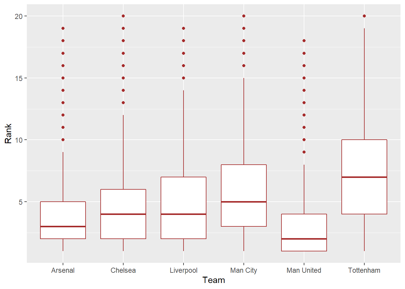
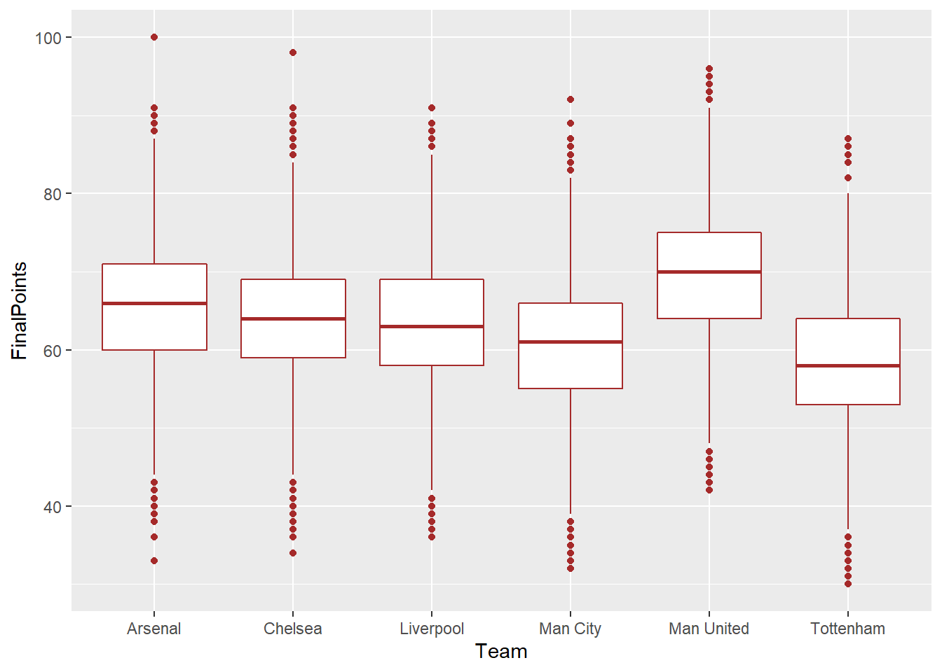
We can see that Man Utd’s rank numbers are lower than other Big 6 clubs on average, meaning that United tend to secure a higher place on the table, and they also have higher mean final points than other teams. In contrast, Tottenham tends to have lower ranking spots and lower points than their fellow Big 6 competitors. Unsurprisingly, there’s a strong and linear correlation between team’s ranks and total points, meaning that higher total points is associated with a higher (lower number) finishing position of the table, as illustrated by the figure below.
EPLSim_All %>%
  group_by(Team) %>%
  summarise(meanPts = mean(FinalPoints),
            meanRank = mean(Rank)) %>%
  ggplot(mapping = aes(meanRank, meanPts)) +
  geom_point() +
  stat_smooth(method = "lm", se = FALSE)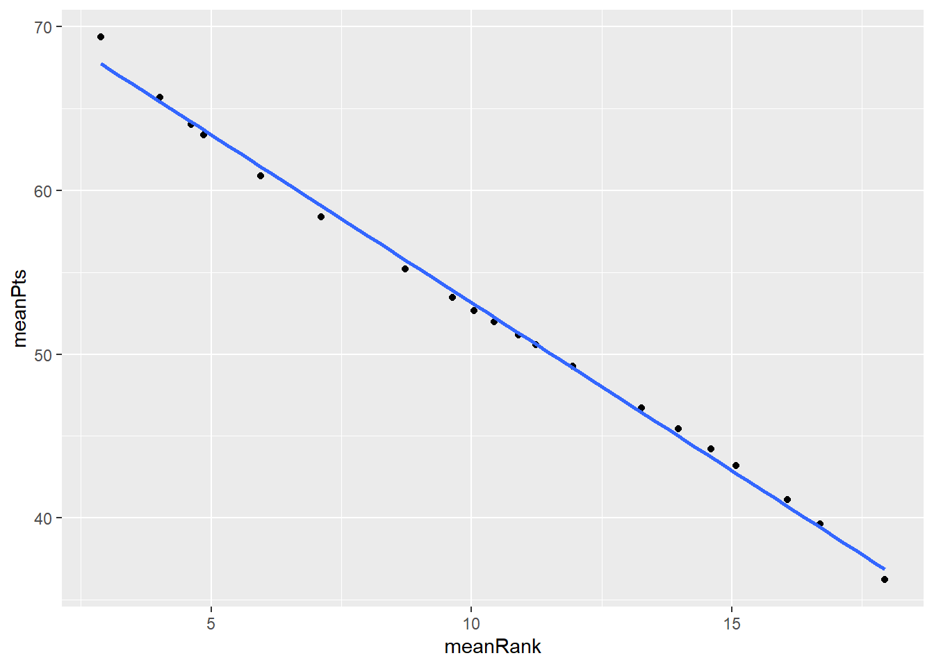
5.1.3.5 Relegation Zone
EPLSim_All %>%
  filter(Rank %in% c(18, 19, 20)) %>%
  group_by(Team) %>%
  summarise(Pct = 100*n()/(nSim)) %>%
  arrange(desc(Pct)) %>%
  head(4) %>%
mykable()| Team | Pct |
|---|---|
| Huddersfield | 69.15 |
| Cardiff | 49.99 |
| Brighton | 41.65 |
| Burnley | 31.60 |
The relegation zone, or the last 3 places on the standings, is where no teams in the Premier League wanted to end up at the end of the season, because this means that the bottom 3 clubs will get relegated to the second highest division of English football (the Championship.) From our simulation results, we see that Huddersfield, Cardiff and Brighton are the 3 squads with the highest chance of being relegated after the 2018-19 season. As a matter of fact, Cardiff and Huddersfield did get relegated at the end of last season, with Fulham being the other member of this group of 3.
5.1.3.6 The 40-point Safety Rule
The 40-point safety rule is an interesting myth related to the EPL’s relegation zone. During the 23 seasons since the league was reduced to 20 clubs (from 1995-96 to 2018-19), there have been only 3 times that a squad got relegated despite hitting the 40-point mark. They are West Ham in 2002-03 with 42 points, and Bolton and Sunderland both with 40 points in 1997-98 and 1996-97 respectively. This mythical 40-point mark has been crucial for the relegation battle for many years, as subpar teams often view getting there as their “security blanket” for remaining in the top division of English football. We’re going to find out if this rule holds well for our simulated results.
EPLSim_All %>%
  filter(Rank %in% c(18,19,20) & FinalPoints >= 40) %>%
  summarise(numSimSeasons = n_distinct(SimNum), numTeams = n()) %>%
mykable()| numSimSeasons | numTeams |
|---|---|
| 3434 | 4424 |
So from our 10000 simulations, 4424 teams could not avoid relegation in spite of reaching the 40-point mark, and 3434 simulations have at least one team that this rule doesn’t work for, so the 40-point safety rule doesn’t hold for 34.34% of the simulated seasons. This percentage is quite high, especially by how rare this phenomenon has actually happened in the history of the league. This could imply that teams in the relegation zone of our simulation results tend to have higher final points than in real life.
EPLSim_All %>%
  filter(Rank %in% c(18,19,20)) %>%
  summarise(AvgFinalPoints = mean(FinalPoints)) %>%
mykable()| AvgFinalPoints |
|---|
| 34.86947 |
Indeed, this is true. The mean point for the bottom 3 teams for our simulations is roughly 35, whereas the 3 relegated clubs last year had 34, 26, and 16 points, which average out to about 25 points.
5.2 Using Data From the 2010s Only
We can now play the same game, but with data coming from a different set of years. This time, we only use data from the previous decade, the 2010s, to predict the results for the 2018-19 season. The simulation is done in a separate script, and after it is complete, the resulting table is written to a csv file.
We now read in the data for further analysis and comparison.
5.3 Using All the Data but Assign More Weight to Recent Seasons
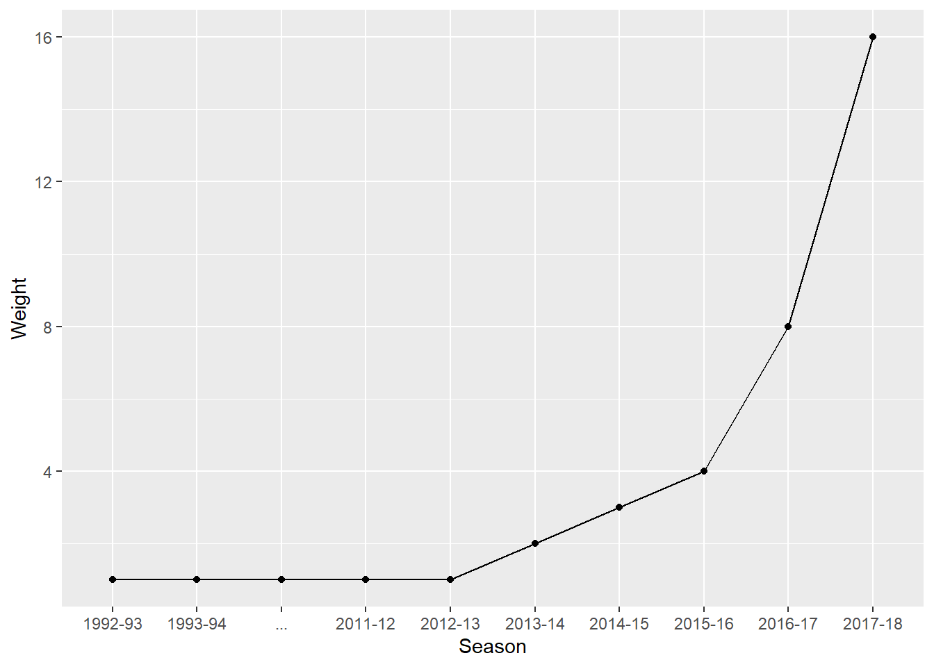
Our third simulation approach is to put more weights towards recent Premier League seasons. This technique is popular in many fields, especially in economics, with the use of assigning more weight to more recent data points in Time series analysis. A common scheme of putting weight to observations is exponential smoothing, where recent cases are given relatively more weight in forecasting than older observations. For this particular simulation method, the way we allocate weight is letting the weight number be equivalent to the number of times the data for a particular season is duplicated. We have decided that the previous 5 years before 2018-19 are almost all that matter. Every season from 1992-93 to 2012-13 are given weight 1, then the weight increases by 1 for each one of 2013-14, 2014-15, and 2015-16. After that we have the 2 most recent years left and we multiply the weight by 2.
The table and graph below illustrate the weight values and the seasons associated with them.
Weights <- tribble( ~Season,  ~Weight,
                    "1992-93", 1,
                    "1993-94", 1,
                    "...", 1,
                    "2011-12", 1,
                    "2012-13", 1,
                    "2013-14", 2,
                    "2014-15", 3,
                    "2015-16", 4,
                    "2016-17", 8,
                    "2017-18", 16)
mykable(Weights) | Season | Weight |
|---|---|
| 1992-93 | 1 |
| 1993-94 | 1 |
| … | 1 |
| 2011-12 | 1 |
| 2012-13 | 1 |
| 2013-14 | 2 |
| 2014-15 | 3 |
| 2015-16 | 4 |
| 2016-17 | 8 |
| 2017-18 | 16 |
We then go on to create a match results table with different weights for each season.
epl9213 <- epl.fulldata[1:8226,] # data from 1992-93 to 2012-13

# get data from epl.season function
# duplicate each season based on its weight
epl1314 <- epl.season(2013)
epl1314 <- epl1314 %>% slice(rep(row_number(), 2))

epl1415 <- epl.season(2014)
epl1415 <- epl1415 %>% slice(rep(row_number(), 3))

epl1516 <- epl.season(2015)
epl1516 <- epl1516 %>% slice(rep(row_number(), 4))

epl1617 <- epl.season(2016)
epl1617 <- epl1617 %>% slice(rep(row_number(), 8))

epl1718 <- epl.season(2017)
epl1718 <- epl1718 %>% slice(rep(row_number(), 16))

eplWt <- epl9213 %>% # join the tables
  full_join(epl1314) %>%
  full_join(epl1415) %>%
  full_join(epl1516) %>%
  full_join(epl1617) %>%
  full_join(epl1718)
After that, we use the exact same simulation process as the previous 2 simulations to get the results for the 2018-19 seasons. As before, after the simulation is finished, we write the simulation table to a csv file. These tasks are done separately in an R script. We now import this data file for further usage in the next section.
5.4 Comparison
We can now look at how our 3 prediction methods differ. We first join the 3 data frames of prediction results together into a table called SimComparison.
Below are the boxplots comparing the Big 6’s rank and final points in each of the 3 simulations. They are followed by a summary table of the big 6’s likelihood of being EPL Champions in each simulation
SimComparison$SimType <-
  factor(SimComparison$SimType,
         levels = c("All Seasons", "2010s", "Assign Weight"))
SimComparison %>%
  filter(Team %in% EPLBig6$Team) %>%
  ggplot(mapping = aes(SimType, Rank)) +
  geom_boxplot() +
  facet_wrap(~ Team)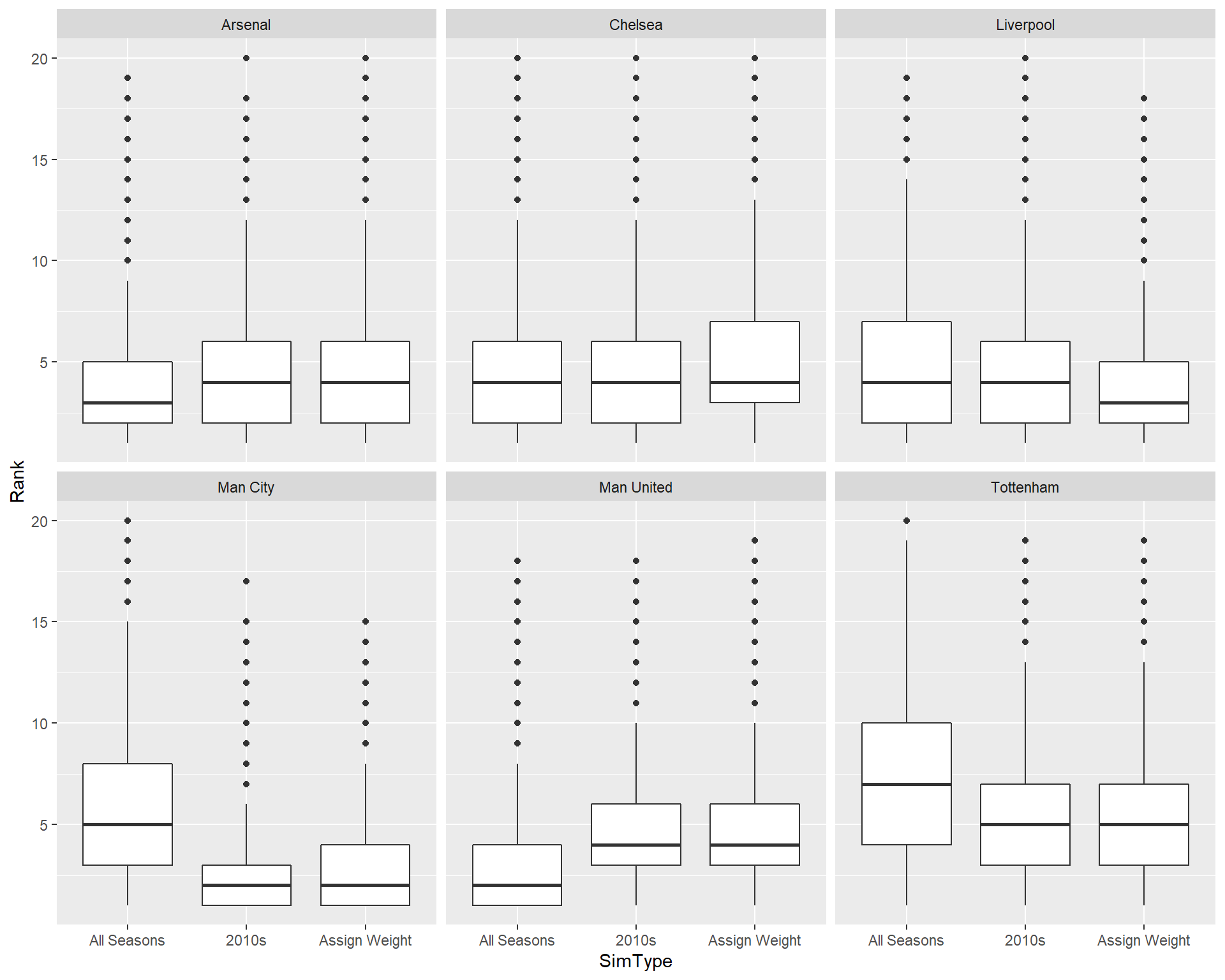
SimComparison %>%
  filter(Team %in% EPLBig6$Team) %>%
  ggplot(mapping = aes(SimType, FinalPoints)) +
  geom_boxplot() +
  facet_wrap(~ Team)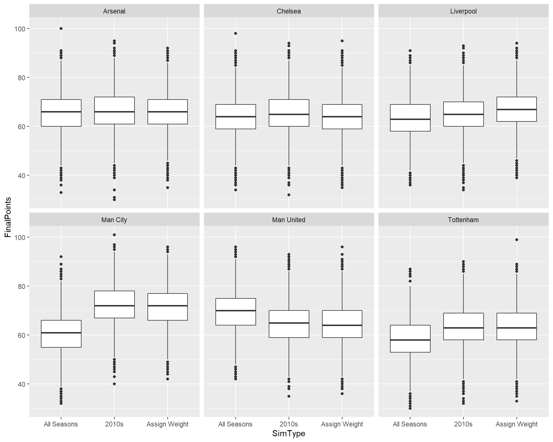
Big6Rank <- SimComparison %>%
  filter(Team %in% EPLBig6$Team) %>%
  filter(Rank == 1) %>%
  group_by(Team, SimType) %>%
summarise(Pct = 100*n()/(nSim))| Team | All Seasons | 2010s | Assign Weight |
|---|---|---|---|
| Arsenal | 19.68 | 15.05 | 14.07 |
| Chelsea | 14.28 | 11.70 | 9.03 |
| Liverpool | 12.50 | 10.96 | 17.61 |
| Man City | 7.00 | 41.71 | 38.09 |
| Man United | 36.99 | 10.47 | 10.53 |
| Tottenham | 3.91 | 7.38 | 8.34 |
Overall, it’s clear that Man Utd’s chance of having higher ranks decreases drastically if we prioritize recent data over just using data from all seasons. Their in-town rivals, Man City, on the other hand, have much higher percentages of winning the league in 2018-19 if we focus on data from recent years. In fact, they were the champions of 2018-19 EPL. Putting weight towards recent years and using only data from the 2010s also lower Chelsea and Arsenal’s likelihood of finishing first, whereas these 2 method increase Tottenham’s chance, though they still have the smallest percentage in each category. Compared to using data from all seasons, Liverpool has lower probability of winning if we take into account the whole 2010s, but higher probability if we use a weighted dataset.
We can compare other things too, like relegation zone outcomes or the 40-point safety rule.
SimComparison %>%
  filter(Rank %in% c(18, 19, 20)) %>%
  group_by(Team, SimType) %>%
  summarise(Pct = 100*n()/(nSim)) %>%
  spread(SimType, Pct) %>%
  arrange(desc(`2010s`)) %>%
mykable()| Team | All Seasons | 2010s | Assign Weight |
|---|---|---|---|
| Huddersfield | 69.15 | 72.91 | 71.03 |
| Cardiff | 49.99 | 54.38 | 53.47 |
| Brighton | 41.65 | 45.03 | 44.03 |
| Burnley | 31.60 | 43.38 | 33.34 |
| Watford | 26.28 | 17.24 | 15.82 |
| Crystal Palace | 17.54 | 14.42 | 10.65 |
| Wolves | 22.04 | 14.22 | 22.32 |
| Newcastle | 2.40 | 8.78 | 7.41 |
| Fulham | 9.87 | 7.91 | 11.74 |
| West Ham | 7.46 | 6.73 | 6.39 |
| Bournemouth | 4.76 | 5.46 | 5.80 |
| Southampton | 6.49 | 5.23 | 11.65 |
| Everton | 3.48 | 2.17 | 3.63 |
| Leicester | 5.53 | 1.75 | 2.39 |
| Tottenham | 1.02 | 0.16 | 0.08 |
| Chelsea | 0.15 | 0.09 | 0.13 |
| Liverpool | 0.10 | 0.05 | 0.02 |
| Man United | 0.01 | 0.05 | 0.04 |
| Arsenal | 0.10 | 0.04 | 0.06 |
| Man City | 0.38 | NA | NA |
The results of the 3 models are pretty consistent with each other, with Huddersfield and Cardiff being the 2 “locks” to play in the lower football division in the following season. Brighton and Burnley also have high chances of being in the bottom 3, although it turned out to be that they got to remain in the league for another year. The third team that got dismissed last year, Fulham, does not have high chances of relegation in any of the 3 simulations. Unsurprisingly, the Big 6’s teams have the smallest chances of getting related. Another interesting result we got from this comparison is Man City never finishes in the bottom 3 if we only use more recent data - data from the 2010s only and putting weight on recent seasons.
SimComparison %>%
  filter(Rank %in% c(18,19,20) & FinalPoints >= 40) %>%
  group_by(SimType) %>%
  summarise(numSimSeasons = n_distinct(SimNum), numTeams = n()) %>%
mykable() | SimType | numSimSeasons | numTeams |
|---|---|---|
| All Seasons | 3434 | 4424 |
| 2010s | 2066 | 2470 |
| Assign Weight | 2346 | 2889 |
Using data from 2010s and assigning weight to recent years give us significantly less number of both teams and seasons that violate the mythical 40-point rule than using all the data. Therefore, we can say that the 40-point safety rule holds much better for the 2 simulations that focus on recent data than the one with data from all previous seasons. This actually quite makes sense, since in the past 2 decades in reality, teams with 40 or more points at the end of a season all survived from relegation, as the last time this rule did not happen was the 1997-98 season.