4 Goal Scoring and the Poisson Process
4.1 The Poisson Process
The Poisson process is a randomly determined process used to model the occurrence (or arrival) of phenomena over a continuous interval, which in most cases represents time. There are several characteristics of the Poisson process that can be observed, including, the number of events happening in a given time period; the time between those events; and when (at what point of time) the events occur. Playing a huge role in the Poisson process is the Poisson distribution, which deals with the number of occurrences of an event in a fixed period of time, with a rate of occurrence parameter \(\lambda\). Another key distribution in this process is the exponential distribution, which has a strong connection with the Poisson distribution, as if the number of occurrences per interval of time are illustrated by Poisson, then the description of the length of time between occurrences are provided by the exponential distribution. If Poisson events take place on average at the rate of \(\lambda\) per unit of time, then the sequence of time between events (or interarrival times) are independent and identically distributed exponential random variables, having mean \(\displaystyle \beta = \frac{1}{\lambda}\). Furthermore, there’s a relationship between Poisson and another famous probability distribution - the continuous uniform distribution. If a Poisson process contains a finite number of events in a given time interval, then the unordered times, or locations, or positions, or points of time at which those events happen are uniformly distributed on that interval.
We suspect that goal scoring in soccer can be modeled by a Poisson process. According to the characteristics described above, if goal scoring for a club happens at a certain rate in a given time period, then a Poisson distribution can be used to model the number of goals scored. Additionally, the waiting time (usually in minutes) between successive instances of goal can be described using an exponential distribution. Moreover, the positions of time, better known as “minute marks”, in a game at which scoring events transpire may be uniformly distributed. We’re going to answer these questions in this research. With that goal, we’re now moving on to the modeling and analysis phases of this report.
4.2 Goal Scoring and the Poisson Distribution
4.2.1 The Poisson Distribution
The Poisson distribution, named for French mathematician Siméon Denis Poisson, is a discrete probability distribution that expresses the number of occurrences of an event over a given period of time. A Poisson random variable can represent many instances in our daily lives such as the number of phone calls coming into the Math Workshop requesting a tutor in a week, the number of misprints in a newspaper, or the number of cars arriving at a fast food drive-through in an hour.
The probability function of a Poisson random variable \(X\) with parameter \(\lambda\) is given by: \[\displaystyle p_X(x) = \frac{{e^{ - \lambda } \lambda ^x }}{{x!}} ; \ x = 0,1,2,... \textrm{ and } \lambda > 0 \] where \(X\) represents the number of occurrences of an event in a given unit time period, and \(\lambda\) is the constant rate of occurrence per time period.
The mean and variance of our Poisson Random Variable \(X\), denoted by \(\mu_X\) and \(\sigma^2_X\) respectively, are \[\mu_X = \lambda\] and \[\sigma^2_X = \lambda\]
We wanted to use this idea to model the goal scoring rate for soccer clubs during the Premier League era.
4.2.2 Poisson and the Number of Goals Scored
We use Manchester United (Man Utd), the most successful English club of all time, as our case of inspection. The question here is “Does Man Utd’s number of goals scored follow a Poisson distribution?” To answer this question, we first create a table of Man Utd’s goals. The table will consist of 2 columns: 1 for how many goals they scored in a match, and 1 for where the match took place - home or away. Therefore, each row of the table represents the number of goals scored in a match and the type of goal.
MUHome <- epl.fulldata %>%
  filter(HomeTeam == "Man United") %>%
  select(Home.Goals) %>%
  mutate(type = "Home") %>%
  rename(goals = Home.Goals) # rename for joining purposes
MUAway <- epl.fulldata %>%
filter(AwayTeam == "Man United") %>%
select(Away.Goals) %>%
mutate(type = "Away") %>%
rename(goals = Away.Goals)We then once again use a full_join to merge our 2 tables into one table.
| goals | type |
|---|---|
| 0 | Home |
| 1 | Home |
| 3 | Home |
We now begin our analysis with a simple histogram and some summary statistics of Man Utd’s goals.
MUGoals %>%
  ggplot(aes(x = goals)) +
  geom_histogram(color = "darkgreen", fill = "lightgreen", bins = 10) +
  scale_x_continuous(breaks= 0:9)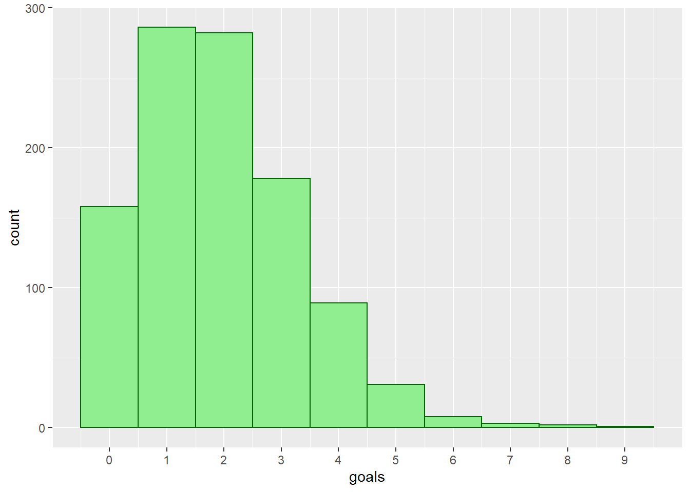
| min | Q1 | median | Q3 | max | mean | sd | n | missing | |
|---|---|---|---|---|---|---|---|---|---|
| 0 | 1 | 2 | 3 | 9 | 1.916185 | 1.405221 | 1038 | 0 |
We now take a look at the mean and variance (the square of the standard deviation) of Man Utd’s scoring rate. We are hoping to see these two values to be equal, since we know that the mean and variance of a Poisson random variable are the same.
MeanGoals <- fav_stats(MUGoals$goals)[[6]]
numMatches <- fav_stats(MUGoals$goals)[[8]]
StDevGoals <- fav_stats(MUGoals$goals)[[7]]
VarianceGoals <- StDevGoals ^ 2## [1] 1.916185## [1] 1.974646The mean and variance of scoring rate are 1.916 and 1.975 respectively, which are pretty close to each other, and this is exactly what we anticipated. We now create a table that will have the possible values for number of goals, along with the following for each value: number of matches, Poisson probability, and expected number of matches. We first compile the number of goals scored and number of matches having those goal values.
GoalsTable <-
  MUGoals %>%
  group_by(goals) %>%
  summarise(ActualMatches = n())
GoalsTable %>%
mykable()| goals | ActualMatches |
|---|---|
| 0 | 158 |
| 1 | 286 |
| 2 | 282 |
| 3 | 178 |
| 4 | 89 |
| 5 | 31 |
| 6 | 8 |
| 7 | 3 |
| 8 | 2 |
| 9 | 1 |
Since there are only a small number of matches with 4 goals or more, it’d be a good idea to combine them into a row called “4 or more.” A more important reason of doing this is we want to meet a technical condition of a Chi-square Goodness of fit test, which we will be conducting shortly. The test is appropriate when the expected value of the number of counts in each level of the variable is at least 5.
# select first 4 rows (0, 1, 2, 3 goals)
NewGoalsTable <- GoalsTable[1:4,]
# sum up the remaining rows
NewGoalsTable[5,] <- sum(GoalsTable[5:nrow(GoalsTable),2])
NewGoalsTable <- mutate(NewGoalsTable, goals = as.character(goals))
# put in 1 category called "4 or more"
NewGoalsTable[5,"goals"] <- "4 or more" | goals | ActualMatches |
|---|---|
| 0 | 158 |
| 1 | 286 |
| 2 | 282 |
| 3 | 178 |
| 4 or more | 134 |
Our next step is to get the Poisson probabilities for our possible goals scored values, using our mean (1.916) as the rate parameter, since we know that the mean of a Poisson distribution is also the event rate \(\lambda\). R’s dpois function, which takes in the values for number of successes and expected number of events, and returns the probability for our value, is used to accomplished this. Since we have a category of “4 or more” goals, in order to calculate this probability, we use the idea of cumulative probability function, which determines the probability that the random variable will be lower than or equal to a value. The ppois function is used, and since we want the probability of 4 or more goals, we find the complement of the probability of 3 or fewer goal.
## [1] 1.916185PoisProb <- dpois(c(0:3), MeanGoals)
PoisProb[5] <- 1 - ppois(3, MeanGoals)
PoisProb <- round(PoisProb, digits = 3)
mykable(PoisProb) | x |
|---|
| 0.147 |
| 0.282 |
| 0.270 |
| 0.173 |
| 0.128 |
## [1] 1We then utilize the Poisson probabilities for each goal value to calculate the expected number of matches associated with those goal categories.
NewGoalsTable <- cbind(NewGoalsTable, PoisProb)
NewGoalsTable <- mutate(NewGoalsTable,
                        ExpectedMatches = round(numMatches * PoisProb))
NewGoalsTable %>%
mykable()| goals | ActualMatches | PoisProb | ExpectedMatches |
|---|---|---|---|
| 0 | 158 | 0.147 | 153 |
| 1 | 286 | 0.282 | 293 |
| 2 | 282 | 0.270 | 280 |
| 3 | 178 | 0.173 | 180 |
| 4 or more | 134 | 0.128 | 133 |
Just by looking at the expected number of matches, we can tell that what was predicted by our model is very similar to the actual number of matches. Furthermore, the bar graph below shows that our model does a pretty great job of predicting the number of matches with each number of goals.
# Graph to compare Expected and Actual Matches
NewGoalsTable %>%
  gather(ActualMatches, ExpectedMatches,
         key = "Type", value = "numMatches") %>%
  ggplot(aes(x = goals, y = numMatches, fill = Type)) +
  geom_bar(stat = "identity", position = "dodge")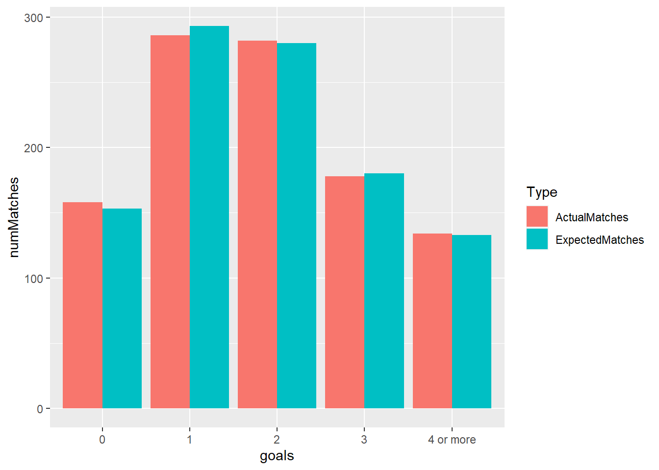
We now conduct a Chi-square Goodness of fit test to confirm that the Man Utd’s actual distribution of goals scored follows a Poisson distribution. The objective of this test is to compare the observed sample distribution with the expected probability distribution (here it’s Poisson.) The null and alternative hypotheses for this test, denoted by \(H_0\) and \(H_A\) respectively, are \(H_0\): the data can be properly modeled by a specified distribution, and \(H_A\): the specified distribution does not fit the data appropriately. For our specific case, the hypotheses are \(H_0\): The distribution of Man Utd’s goals scored follows a Poisson distribution, and \(H_A\): The distribution of Man Utd’s goals scored does not follow a Poisson distribution.
The Chi-square test statistics (\(\chi^2\) ) is defined by the following formula:
\[\displaystyle \chi^2 = \sum_{i} \frac{(O_{i} - E_{i})^2}{E_i}\]
where \(O_{i}\) is the observed number of observations in category \(i\), and \(E_{i}\) is the expected number of observations in category \(i\). In our case, we have 5 total categories for goals scored: 0, 1, 2, 3, and 4 or more. The p-value for the Chi-square Goodness of fit test can be obtained from the upper tail of a Chi-square distribution of the \(\chi^2\) statistics on \(k - 1\) degrees of freedom, where \(k\) is the number of categories. Fortunately for us, R has a function to perform a Chi-square test. We use the function chisq.test to find out how well the Poisson distribution fits our data.
MUChisq <- chisq.test(NewGoalsTable$ActualMatches,
                      p = NewGoalsTable$PoisProb, rescale.p = TRUE)
MUChisq
##
## Chi-squared test for given probabilities
##
## data: NewGoalsTable$ActualMatches
## X-squared = 0.3805, df = 4, p-value = 0.984Since we get a very large p-value (0.984), we do not reject the null hypothesis of our Chi-square test. So we don’t have evidence to claim that the data don’t fit a Poisson distribution. We now use the idea of the power of a hypothesis test to make a final conclusion. The power of a test is the probability that it will correctly reject a false null hypothesis. It is highly influenced by the test’s sample size, the larger the number of observations, the higher the statistical power of a test. Since we have a large sample size of 1038 Man Utd’s games here, it is safe to say that our Chi-square goodness of fit test has high power. Hence we can conclude that there is no significant difference between the data’s and expected distribution. Thus the distribution of Man Utd’s goal scoring data is consistent with a Poisson distribution.
We can now put together everything we just did and create a function to check whether any Premier League team’s goal scoring distribution can be modeled by a Poisson process.
PoissonFit <- function(Team){
  TeamHome <- epl.fulldata %>%
    filter(HomeTeam == Team) %>%
    select(Home.Goals) %>%
    mutate(type = "Home") %>%
    rename(goals = Home.Goals)

  TeamAway <- epl.fulldata %>%
    filter(AwayTeam == Team) %>%
    select(Away.Goals) %>%
    mutate(type = "Away") %>%
    rename(goals = Away.Goals)

  TeamGoals <- full_join(TeamHome, TeamAway, by = c("goals","type"))
  MeanGoals <- fav_stats(TeamGoals$goals)[[6]]
  numMatches <- fav_stats(TeamGoals$goals)[[8]]

  GoalsTable <- TeamGoals %>%
    group_by(goals) %>%
    summarise(ActualMatches = n())

  NewGoalsTable <- GoalsTable[1:4,]
  NewGoalsTable[5,] <- sum(GoalsTable[5:nrow(GoalsTable),2])
  NewGoalsTable <- mutate(NewGoalsTable, goals = as.character(goals))
  NewGoalsTable[5,"goals"] <- "4 or more"

  PoisProb <- dpois(c(0:3), MeanGoals)
  PoisProb[5] <- 1 - ppois(3, MeanGoals)
  PoisProb <- round(PoisProb, digits = 3)
  ExpectedMatches <- as.integer(numMatches * PoisProb)
  NewGoalsTable <- cbind(NewGoalsTable, PoisProb, ExpectedMatches)
}
Let’s take a look at how consistent Tottenham’s goals scored distribution is with the Poisson distribution.
| goals | ActualMatches | PoisProb | ExpectedMatches |
|---|---|---|---|
| 0 | 244 | 0.225 | 233 |
| 1 | 359 | 0.336 | 348 |
| 2 | 233 | 0.250 | 259 |
| 3 | 124 | 0.124 | 128 |
| 4 or more | 78 | 0.064 | 66 |
TotChisq <- chisq.test(TotGoalsTable$ActualMatches,
                       p = TotGoalsTable$PoisProb, rescale.p = TRUE)
TotChisq
##
## Chi-squared test for given probabilities
##
## data: TotGoalsTable$ActualMatches
## X-squared = 5.6541, df = 4, p-value = 0.2265A \(\chi^2\) value of 5.545 and a p-value of 0.236 tell us there’s no evidence to conclude that Tottenham’s data don’t follow a Poisson distribution. Similary to Man Utd, due to a large sample size of Spurs’ games, we can safely draw a conclusion that their goals scored can be modeled by a Poisson distribution.
Again, with this function, we can play the same game with other clubs. While the Poisson distribution fits the goal scoring data for the two teams we just looked at, this is not the case for all Premier League clubs. For instance, if we examine Liverpool…
| goals | ActualMatches | PoisProb | ExpectedMatches |
|---|---|---|---|
| 0 | 225 | 0.181 | 187 |
| 1 | 293 | 0.309 | 320 |
| 2 | 248 | 0.264 | 274 |
| 3 | 158 | 0.151 | 156 |
| 4 or more | 114 | 0.095 | 98 |
LivChisq <- chisq.test(LivGoalsTable$ActualMatches,
                       p = LivGoalsTable$PoisProb, rescale.p = TRUE)
LivChisq
##
## Chi-squared test for given probabilities
##
## data: LivGoalsTable$ActualMatches
## X-squared = 14.619, df = 4, p-value = 0.00556our test results of \(\chi^2\) = 14.62 and a small p-value of 0.0056 indicate that Liverpool’s data is not consistent with the Poisson distribution. One possible explanation of why this does not work for Liverpool is their scoring rate is not constant throughout the years, whereas constant occurrence rate is a necessary condition for a Poisson random variable.
4.3 Time Between Goals and the Exponential Distribution
4.3.1 The Exponential Distribution
The exponential distribution is closely related to the Poisson distribution that was discussed in the previous section. Recall that the Poisson process is used to model some random and sporadically occurring event in which the mean, or rate of occurrence (per time unit) is \(\lambda\). In the last chapter, we used the Poisson distribution to model goal scoring rate per match for Man United, and since we only focused on integer goal values, our Poisson random variable is discrete. We are now interested in modeling the time until the next occurrence of goal, which we can also think of in terms of “time between goals”. If we have a non-negative random variable \(X\) that is the time until the next occurrence in a Poisson process, then X follows an exponential distribution with probability density function
\[\displaystyle f_X(x) = \lambda e^{-\lambda x} = \frac{1}{\beta} e^{-\frac{1}{\beta} x}; \ x \ge 0\]
where \(\lambda\) represents the average rate of occurrence and \(\beta\) is the average time between occurrences.
The mean and variance of an exponentially distributed random variable X are \[\displaystyle \mu_X = \frac{1}{\lambda} = \beta\] and \[\displaystyle \sigma^2_X = \frac{1}{\lambda^2} = \beta^2\] We’re going to use this idea to model the time between each goal for a Premier League team in a given season.
4.3.2 Time Between Goals
For this analysis, we use the muscoringtime.xlsx data file, as mentioned in the data importing section of this report. This data file contains 5 columns: Minutes, which is the point of time during a match at which a goal was scored; Matchweek, which is the fixture number of each game; the stoppage time in minutes for both halves of each game, and finally, the time between goals, which takes into account the stoppage time. We collected these 5 variables for all Man Utd’s goals during their 2018-19 Premier League campaign. Here’s a quick glance at our data table after we read in the data file.
| Min | Matchweek | H1_stoppage | H2_stoppage | TimeBetween |
|---|---|---|---|---|
| 3 | 1 | 2 | 5 | 0 |
| 83 | 1 | 2 | 5 | 82 |
| 34 | 2 | 5 | 6 | 46 |
| 95 | 2 | 5 | 6 | 66 |
We’re going to take a moment to explain some of the above table’s attributes. In soccer, the term “stoppage time” is used to describe the number of minutes added to the end of each half to help make up for time lost during the course of the half, due to various reasons such as fouls, injuries, players and referees arguments, or goal celebrations, for all of which the game is not being played. The variable of time between goals is calculated by measuring the minutes between a goal and the goal before it in the season. For example, if we look at row 3 of the above table, the value of TimeBetween is 46. We note that this goal was scored at the 34th minute mark of matchweek 2, and the goal before it was being put in the back of the net at minute 83 of matchweek 1. Since the 90th minute signifies the end of the second half, there are 7 minutes between the moment Man Utd last scored (83th minute) and when the half should theoretically end. Furthermore, because we also take into account stoppage time, we have to add the 5 added minutes to the second half of matchweek 2’s game. Finally, we add 7, 5, and 34 together to get 46 minutes of time between these 2 goals.
As usual, we start off our data analysis with some basic visual and numerical summaries of our data. Below are a histogram and some descriptive statistics of Man Utd’s time between each goal last season.
muscoringtime %>%
  filter(!is.na(TimeBetween)) %>%
  ggplot() +
  geom_histogram(mapping = aes(TimeBetween), color = "darkgreen",
                 fill = "lightgreen", breaks = seq(1,300, by = 20))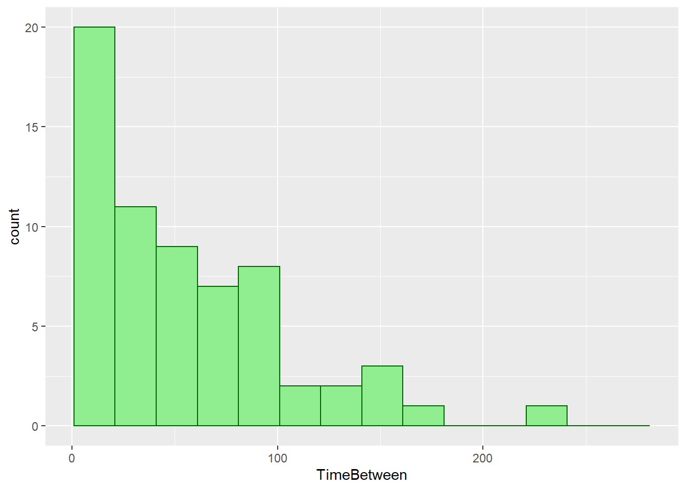
| min | Q1 | median | Q3 | max | mean | sd | n | missing | |
|---|---|---|---|---|---|---|---|---|---|
| 0 | 17 | 43 | 82 | 236 | 54.72308 | 47.75769 | 65 | 7 |
The overall shape of this histogram looks like an exponential distribution curve, which is a continuous, smooth and concave up graph, displaying exponential decay. This is a good sign for us, since we suspected that time between goals for Man Utd is exponentially distributed.
Now we’re going to compare 1/(mean time between), which is the Poisson rate of occurrence \(\lambda\), and 1/(standard deviation of time between). We are hoping that these 2 values are equal to each other, since for an exponentially distributed random variable, its variance is equal to its mean squared, and we also know that standard deviation is the square root of variance, so mean and standard deviation should be equal, and so are their reciprocals.
## [1] 0.01827383## [1] 0.02093904The values are not that far away, which leads us to believe more that our initial suspicion is true.
Just like the previous section with the Poisson distribution, we would like to know whether the time between goals of Man Utd follows an exponential distribution. To check this, we perform a Kolmogorov-Smirnov (KS) test, which is another Goodness of fit test. This KS test applies to continuous distributions, like our distribution of interest, exponential; whereas the Chi-square test we used in the previous section works best for categorized data, meaning that the data has been counted and divided into categories. Named after two Soviet mathematicians Andrey Kolmogorov and Nikolai Smirnov, the KS test compares the data with a known distribution and tells us if they have the same distribution. The null and alternative hypotheses for this test are: Ho: the data follow a specified distribution (in our case, the minutes between goal follow an exponential distribution), and Ha: the data do not follow the specified distribution.
The test statistic for a KS test is defined as
\[D = \max_{x} |F_{n}(x) - F(x)|\]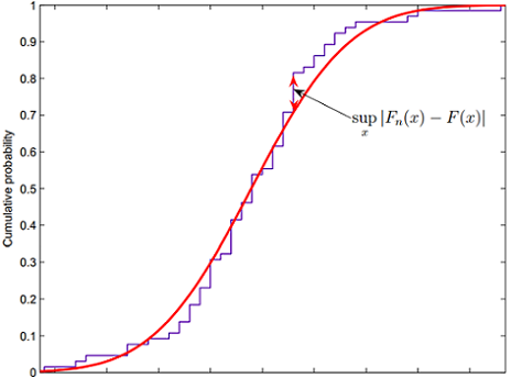
As shown in the figure above, this D value represents the greatest vertical distance, denoted by max for maximum (or sometimes by sup for supremum) between the empirical distribution function of the sample and the cumulative distribution function of the reference distribution (here it’s exponential.) The closer (or lower) the D value to zero, the more probable that the data follow the specified distribution. The higher D is to 1, the more probable that they have different distributions.
We once again take advantage of a built-in function in R that performs a KS test for us. The function ks.test is used, which takes in the data and the distribution (with its parameter(s) fully specified) we want do compare our data with, and gives us the KS test statistics D and also a p-value of the test. We also create a graph to compare the cumulative distributions of time between goals and the hypothetical distribution - the exponential.
##
##  One-sample Kolmogorov-Smirnov test
##
## data:  muscoringtime$TimeBetween
## D = 0.089216, p-value = 0.6789
## alternative hypothesis: two-sided
x <- muscoringtime$TimeBetween
plot(ecdf(x), xlab = "Time Between",
ylab = "Cumulative Distribution", main = "", pch = 20)
curve((1 - exp(-(1/MeanTimeBetween)*x)), 0, 240, add = TRUE, col = "blue")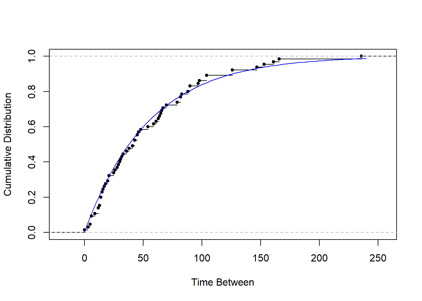
Since we get D = 0.089 and p-value = 0.679, we fail to reject the null hypothesis. Thus there’s not sufficient evidence to support a conclusion that our data are not consistent with the exponential distribution. For this test, since we have a large enough number of data values, the test has high statistical power, and this allows us to say that the time between goals of Man Utd follows an exponential distribution.
4.4 Scoring Time and the Uniform Distribution
4.4.1 The Continuous Uniform Distribution
The continuous uniform distribution is a probability distribution with equally likely outcomes, meaning that its probability density is the same at each point in an interval \([A,B]\). The graph of a uniform distribution results in a rectangular shape, hence this is why it is sometimes referred to as the “rectangular distribution.”
A continuous random variable X is uniformly distributed on \([A,B]\) if its probability density function is defined by
\[\displaystyle f_X(x) = \frac{1}{B-A}; \ A \le x \le B\]
The mean and variance of a uniformly distributed random variable X are
\[\displaystyle \mu_X = \frac{A + B}{2}\] and \[\displaystyle \sigma^2_X = \frac{(B-A)^2}{12}\]
One popular version of the uniform distribution is the standard uniform distribution. The domain for this special case is the unit interval \([0,1]\). A random variable U is said to have a standard uniform distribution if it has probability density function
\[f(u) = 1; \ 0 \le u \le 1\]
The mean and variances of U on \([0,1]\) are \[\displaystyle \mu_U = \frac{1}{2}\] and \[\displaystyle \sigma^2_U = \frac{1}{12}\]
We suspect that the scoring time of Man Utd is uniformly distribution. To that end, let’s find out whether this is true.
4.4.2 Are the Scoring Time Uniformly Distributed?
We first standardize the minutes by dividing each one of them by the total minutes of their respective game. The reason for standardizing the minutes is because the match total time varies, since we also take into account the stoppage time, which means some matches lasted longer than others.
MUTime <- muscoringtime %>%
  filter(!is.na(Min)) %>%
  mutate(StdMin = Min/(90 + H1_stoppage + H2_stoppage))
Below are a histogram and some summary statistics of the standardized version of Man Utd’s scoring minutes last season.
MUTime %>%
  ggplot() +
  geom_histogram(mapping = aes(StdMin), color = "darkgreen",
                 fill = "lightgreen", breaks = seq(0, 1, by=0.1))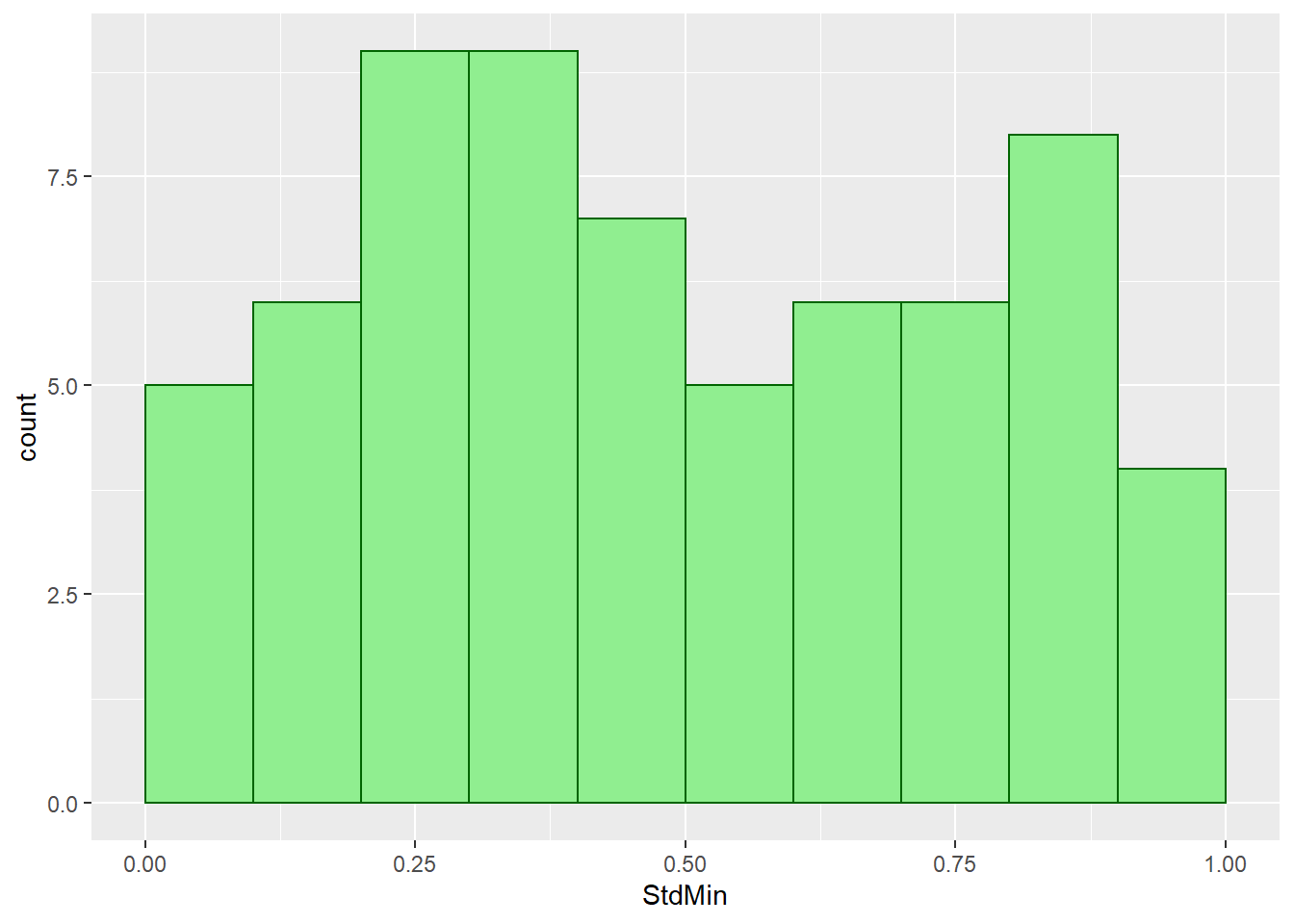
| min | Q1 | median | Q3 | max | mean | sd | n | missing | |
|---|---|---|---|---|---|---|---|---|---|
| 0.031 | 0.289 | 0.444 | 0.727 | 0.941 | 0.4882769 | 0.2707408 | 65 | 0 |
The overal shape of the distribution of standardized minutes is not as rectangular as the usual uniform curve. What we can tell from this distribution is goals tend to occur in the middle minutes of each half, and less goals take place at the beginning and end of each playing period. We now compare the mean and variance of standardized scoring minutes of our data with the mean and variance of a standard uniform distribution, which are \(\frac{1}{2}\) and \(\frac{1}{12}\) respectively.
## [1] 0.4882443## [1] 0.5## [1] 0.07331052## [1] 0.08333333Our data’s mean is pretty close to the expected value for a standard uniform random variable. Meanwhile, our variance value is slightly smaller than the expected variance. One possible explanation for this low variance value is because our distribution graph is not as flat as the regular uniform curve, as we observed more goals toward the middle and fewer goals than expected at the extremes of the distribution. Thus this means the goal data points are closer to the center, which results in a narrower spread.
Just like before, we are interested in finding out whether our data of Man Utd’s scoring time actually follow a standard uniform distribution. Since our distribution is continuos, we once again use a Kolmogorov-Smirnov goodness of fit test to answer this question. Just like the KS test from the previous section, the null hypothesis for this test is there’s a good fit between our data and the specified distribution (uniform in this case), and the alternative hypothesis is the scoring time data don’t fit the uniform distribution. The test results are accompanied by a plot showing how the empirical and hypothetical cumulative distributions differ.
##
##  One-sample Kolmogorov-Smirnov test
##
## data:  MUTime$StdMin
## D = 0.085385, p-value = 0.7305
## alternative hypothesis: two-sided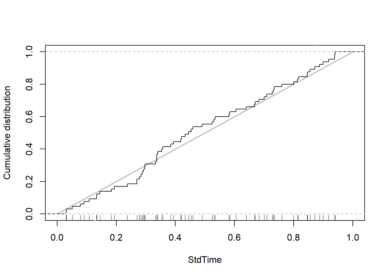
A D-statistics of 0.0854 and a p-value of 0.73 indicate that there’s no good evidence against the claim that the data is not consistent with a uniform distribution. Similar to our previous goodness-of-fit tests, because we have a big enough amount of data points leading to high statistical power here, we can conclude that our data is consistent with the specified reference distribution. In context, the standardized scoring time for Man Utd during the 2018-19 season is uniformly distributed.