4 Classification

But in many situations, the response variable is instead qualitative. For example, eye color is qualitative. Often qualitative variables are referred to as categorical; we will use these terms interchangeably. In this chapter, we study approaches for predicting qualitative responses, a process that is known as classification.

The methods covered in this chapter include logistic regression (and Poisson regression), linear discriminant analysis, quadratic discriminant analysis, naive Bayes, and \(K\)-nearest neighbors.

4.1 An Overview of Classification

In this chapter, we will illustrate the concept of classification using the simulated Default data set. We are interested in predicting whether an individual will default on his or her credit card payment, on the basis of annual income and monthly credit card balance.

Load the go-to packages and the default data set:

library(tidyverse)
library(broom)
library(gt)
library(patchwork) # for composing plots
library(tictoc) # for timing code execution

# Load my R package and set the ggplot theme
library(dunnr)
extrafont::loadfonts(device = "win", quiet = TRUE)
theme_set(theme_td())
set_geom_fonts()
set_palette()

default <- ISLR2::Default
glimpse(default)

## Rows: 10,000
## Columns: 4
## $ default <fct> No, No, No, No, No, No, No, No, No, No, No, No, No, No, No, No…
## $ student <fct> No, Yes, No, No, No, Yes, No, Yes, No, No, Yes, Yes, No, No, N…
## $ balance <dbl> 729.5265, 817.1804, 1073.5492, 529.2506, 785.6559, 919.5885, 8…
## $ income  <dbl> 44361.625, 12106.135, 31767.139, 35704.494, 38463.496, 7491.55…

Randomly choose a subset of the 10000 observations and re-create Figure 4.1:

d <- default %>%
  add_count(default, name = "n_group") %>%
  slice_sample(
    n = 1000,
    # Inversely weight by group size to get more even distribution
    weight_by = n() - n_group
  )
p1 <- d %>%
  ggplot(aes(x = balance, y = income)) +
  geom_point(aes(color = default, shape = default),
             alpha = 0.5, show.legend = FALSE)
p2 <- d %>%
  ggplot(aes(x = default, y = balance)) +
  geom_boxplot(aes(fill = default), show.legend = FALSE)
p3 <- d %>%
  ggplot(aes(x = default, y = income)) +
  geom_boxplot(aes(fill = default), show.legend = FALSE)
p1 | (p2 | p3)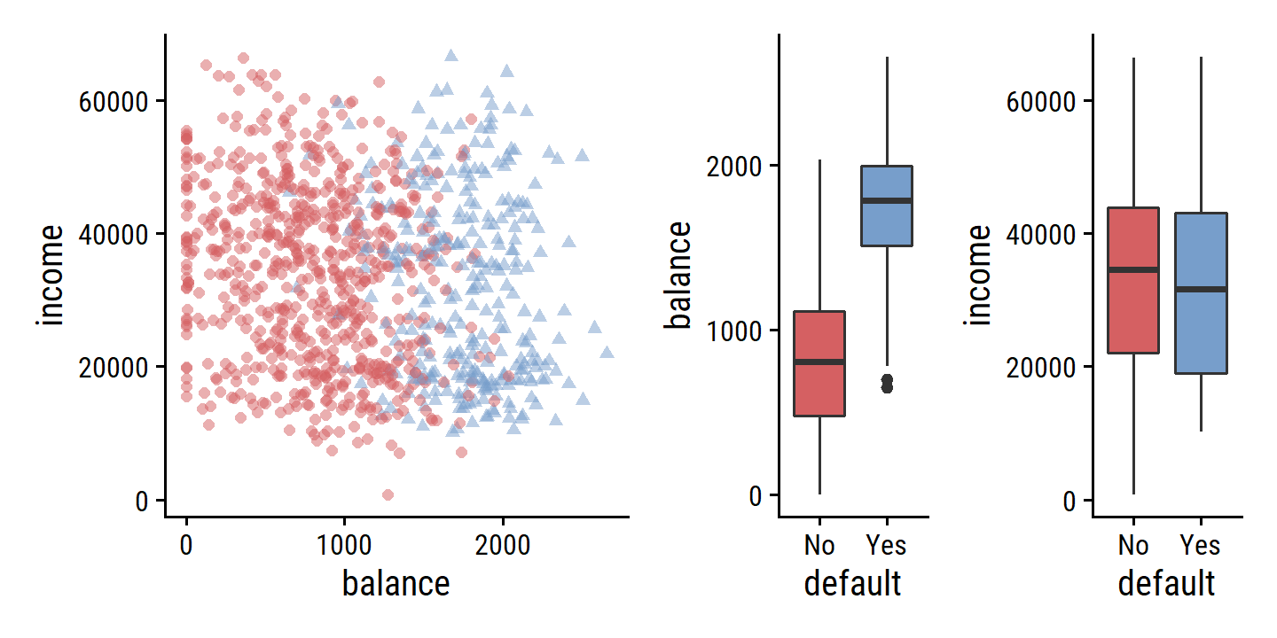

4.2 Why Not Linear Regression?

Linear regression cannot predict un-ordered qualitative responses with more than two levels.

Unfortunately, in general there is no natural way to convert a qualitative response variable with more than two levels into a quantitative response that is ready for linear regression.

It is possible to use linear regression to predict a binary (two level) response. For example, if we code stroke and drug overdose as dummy variables:

\[ Y = \begin{cases} 0 & \text{if stroke;} \\ 1 & \text{if drug overdose}. \end{cases} \]

Then we predict stroke if \(\hat{Y} <= 0.5\) and overdose if \(\hat{Y} > 0.5\). It turns out that these probability estimates are not unreasonble, but there can be issues:

However, if we use linear regression, some of our estimates might be outside the [0, 1] interval (see Figure 4.2), making them hard to interpret as probabilities! Nevertheless, the predictions provide an ordering and can be interpreted as crude probability estimates.

4.3 Logistic Regression

In logistic regression, we model the probability of \(Y\) belonging to a class, rather than the response \(Y\) itself. The probability of default given balance can be written:

\[ \text{Pr}(\text{default = Yes}|\text{balance}) = p(\text{balance}). \]

One might predict a default for an individual with \(p(\text{balance}) > 0.5\). Or they may alter the threshold to be conservative, e.g. \(p(\text{balance}) > 0.1\)

4.3.1 The Logistic Model

As previously discussed, we could model the probability as linear:

\[ p(X) = \beta_0 + \beta_1 X \]

but this could give probabilities outside of the range 0-1. We must instead model \(p(X)\) using a function that gives outputs 0-1. Many functions meet this description, but logistic regression uses the logistic function:

\[ p(X) = \frac{e^{\beta_0 + \beta_1X}}{1 + e^{\beta_0 + \beta_1 X}}. \]

Fit the linear and logistic probability models and re-create Figure 4.2:

lm_default_balance <-
  lm(
    default ~ balance,
     # Turn the factor levels into 0 and 1
    data = default %>% mutate(default = as.numeric(default) - 1)
  )
glm_default_balance <-
  glm(default ~ balance, data = default,
      family = binomial(link = "logit"))
# Plot the data
p <- default %>%
  ggplot(aes(x = balance)) +
  geom_point(aes(y = as.numeric(default) - 1), color = td_colors$nice$soft_orange, alpha = 0.5)
# Plot the linear model
p1 <- p +
  geom_abline(slope = coef(lm_default_balance)["balance"],
              intercept = coef(lm_default_balance)["(Intercept)"],
              size = 1.5, color = td_colors$nice$strong_blue) +
  labs(y = "Probability of default")
# Plot the logistic model
p2 <- p +
  geom_line(
    aes(y = pred_default),
    data = tibble(balance = seq(0, 2700, 1)) %>%
      mutate(
        sum_beta = coef(glm_default_balance)["(Intercept)"] +
                       balance * coef(glm_default_balance)["balance"],
        pred_default = plogis(sum_beta)
      ),
    size = 1.5, color = td_colors$nice$strong_blue
  ) +
  labs(y = NULL)
p1 | p2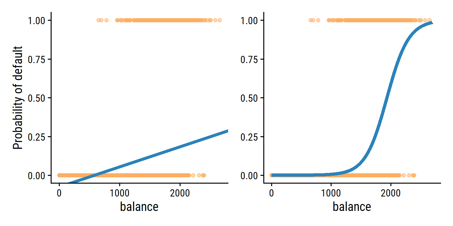

A very clear improvement. The mean of the fitted probabilities in both models return the overall proportion of defaulters in the data set:

predict(lm_default_balance, newdata = default) %>%
  mean()

## [1] 0.0333

predict(glm_default_balance, newdata = default) %>%
  plogis() %>%
  mean()

## [1] 0.0333

The odds is found by re-arranging the logistic function:

\[ \frac{p(X)}{1 - p(X)} = e^{\beta_0 + \beta_1 X}. \]

This can take any value between 0 (\(p(X) = 0\)) and \(\infty\) (\(p(X) = 1\)). Basic interpretation:

• A probability of 0.2 gives 1:4 odds.
• A probability of 0.9 gives 9:1 odds.

Taking the logarithm of both sides gives us the log odds or logit which is linear in \(X\):

\[ \log \left(\frac{p(X)}{1 - p(X)}\right) = \beta_0 + \beta_1 X. \] A one unit change in \(X\) increases the log odds by \(\beta_1\). Equivalently, it multiplies the odds by \(e^{\beta_1}\).

4.3.2 Estimating the Regression Coefficients

We fit logistic regression models with maximum likelihood, which seeks estimates for \(\beta_0\) and \(\beta_1\) such that the predicted probabilities \(\hat{p}(x_i)\) corresponds as closely as possible to the values \(y_i\). This idea is formalized using a likelihood function:

\[ \ell (\beta_0, \beta_1) = \prod_{i: y_i = 1} p(x_i) \prod_{i': y_{i'} = 0} (1 - p(x_{i'})). \]

We find the estimates \(\hat{\beta}_0\) and \(\hat{\beta}_1\) by maximizing this likelihood function. Note that the least squares approach to linear regression is a special case of maximum likelihood.

Re-produce Table 4.1 using the fitted model:

# Since I will be reproducing this table often, write a function
tidy_custom <- function(mod, coef_round = 4, se_round = 4, z_round = 2) {
  tidy(mod) %>%
    transmute(
      term,
      coefficient = round(estimate, coef_round),
      std.error = round(std.error, se_round),
      `z-statistic` = round(statistic, z_round),
      `p-value` = scales::pvalue(p.value)
    )
}
tidy_custom(glm_default_balance) %>% gt() 

term	coefficient	std.error	z-statistic	p-value
(Intercept)	-10.6513	0.3612	-29.49	<0.001
balance	0.0055	0.0002	24.95	<0.001

The \(z\)-statistic plays the same role at the \(t\)-statistic from linear regression. It equals \(\hat{\beta}_1 / \text{SE}(\hat{\beta}_1)\) and large (absolute) values indiciate evidence against the null hypothesis \(H_0: \beta_1 = 0\). The small \(p\)-value associated with balance in the above table is small, so we reject the null hypothesis.

4.3.3 Making Predictions

With the estimates, we can compute default probabilities for an individual with a balance of $1,000 and $2,000.

example_balance <- c(1000, 2000)
# For convenience, add together the linear terms to get the log-odds
sum_beta <- coef(glm_default_balance)["(Intercept)"] +
  example_balance * coef(glm_default_balance)["balance"]

exp(sum_beta) / (1 + exp(sum_beta))

## [1] 0.005752145 0.585769370

Instead of manually writing out the full equation, here are some alternatives:

This logistic distribution function stats::plogis (sometimes called the inverse logit) returns probabilities from the given log-odds values:

stats::plogis(sum_beta)

## [1] 0.005752145 0.585769370

Calling the generic predict on a glm uses predict.glm():

# By default, predict.glm() returns log-odds
predict(glm_default_balance,
        newdata = tibble(balance = example_balance)) %>%
  # So use the inverse logit
  plogis()

##           1           2 
## 0.005752145 0.585769370

There is an argument to predict.glm() called type that specifies the scale of the returned predictions. By default, type = “link” which refers to the link function which means log-odds are returned. Setting type = “response” returns probabilities:

predict(glm_default_balance, newdata = tibble(balance = example_balance),
        type = "response")

##           1           2 
## 0.005752145 0.585769370

Fit the model with student as the predictor and re-create Table 4.2:

glm_default_student <-
  glm(default ~ student, data = default,
      # Note: don't need to specify binomial(link = "logit") because it is the
      #  default link
      family = binomial)
tidy_custom(glm_default_student) %>% gt()

term	coefficient	std.error	z-statistic	p-value
(Intercept)	-3.5041	0.0707	-49.55	<0.001
studentYes	0.4049	0.1150	3.52	<0.001

The probabilities for student and non-students:

predict(glm_default_student, newdata = tibble(student = c("Yes", "No")),
        type = "response")

##          1          2 
## 0.04313859 0.02919501

4.3.4 Multiple Logistic Regression

The extension to multiple predictors \(p\) is straightfoward:

\[ \log \left( \frac{p(X)}{1 - p(X)} \right) = \beta_0 + \beta_1 X_1 + \dots + \beta_p X_p. \]

Fit the model with all three predictors (income in thousands of dollars):

glm_default_all <-
  glm(default ~ .,
      data = default %>% mutate(income = income / 1000),
      family = binomial)
tidy_custom(glm_default_all) %>% gt()

term	coefficient	std.error	z-statistic	p-value
(Intercept)	-10.8690	0.4923	-22.08	<0.001
studentYes	-0.6468	0.2363	-2.74	0.006
balance	0.0057	0.0002	24.74	<0.001
income	0.0030	0.0082	0.37	0.712

The coefficient for student is statistically significant and negative, whereas it was positive in the univariable model. To understand this apparent paradox, re-create Figure 4.3:

balance_breaks <- seq(0, 2700, by = 270)
balance_midpoints <-
  (balance_breaks[1:(length(balance_breaks) - 1)] +
     balance_breaks[2:length(balance_breaks)]) / 2
p1 <- default %>%
  mutate(
    balance_binned = cut(balance, breaks = balance_breaks,
                         include.lowest = TRUE, labels = balance_midpoints),
    balance_binned = as.numeric(as.character(balance_binned))
  ) %>%
  group_by(student, balance_binned) %>%
  summarise(p_default = mean(default == "Yes"), .groups = "drop") %>%
  ggplot(aes(x = balance_binned, y = p_default, color = student)) +
  geom_line(size = 1.5) +
  geom_hline(
    data = default %>%
      group_by(student) %>%
      summarise(p_mean_default = mean(default == "Yes"),
                .groups = "drop"),
    aes(yintercept = p_mean_default, color = student), lty = 2, size = 1
  ) +
  scale_color_manual(values = c(td_colors$nice$strong_blue,
                                td_colors$nice$strong_red)) +
  theme(legend.position = c(0.2, 0.7))
p2 <- default %>%
  ggplot(aes(x = student, y = balance)) +
  geom_boxplot(aes(fill = student)) +
  scale_fill_manual(values = c(td_colors$nice$strong_blue,
                                td_colors$nice$strong_red)) +
  theme(legend.position = "none")
p1 | p2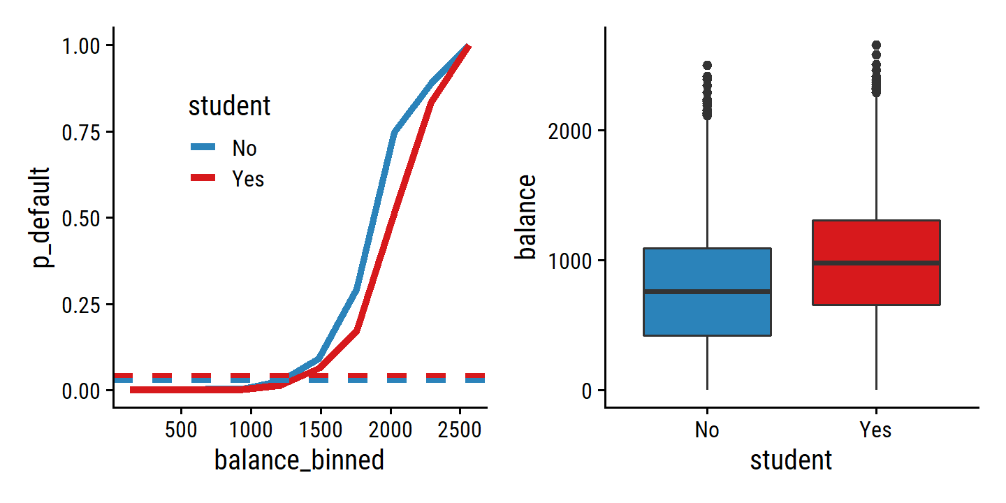

In the left panel, we see that students have a higher overall default rate (4.3%) than non-students (2.9%) as shown by the dashed lines. This is why, in the univariable regression, student was associated with an increase in probability of default. But by the solid lines, we see that for most values of balance, students have lower default rates. And that is what the multiple logistic regression model tells us: for fixed values of balance and income, a student is less likely to default.

This is explained by the right panel above: student and balance are correlated in that students tend to hold higher levels of debt, which is then associated with higher probability of default.

Taken altogether, we can conclude that a student is less likely to default than a non-student with the same credit card balance. Without any information about their balance, however, a student is more likely to default because they are also more likely to carry a higher balance.

This simple example illustrates the dangers and subtleties associated with performing regressions involving only a single predictor when other predictors may also be relevant. As in the linear regression setting, the results obtained using one predictor may be quite different from those obtained using multiple predictors, especially when there is correlation among the predictors. In general, the phenomenon seen in Figure 4.3 is known as confounding.

Make predictions for a student and non-student:

d <- tibble(
  student = c("Yes", "No"), balance = 1500,
  # Income in thousands
  income = 40000 / 1000
)
predict(glm_default_all, newdata = d, type = "response")

##          1          2 
## 0.05788194 0.10499192

4.3.5 Multinomial Logistic Regression

For predicting \(K > 2\) classes, we can extend logistic regression in a method called multinomial logistic regression. To do this, we choose a single class \(K\) to serve as the baseline. Then the probability of another class \(k\) is:

\[ \text{Pr}(Y = k|X = x) = \frac{e^{\beta_{k0} + \beta_{k1} x_1 + \beta_{kp} x_p}}{1 + \sum_{l=1}^{K-1} e^{\beta_{l0} + \beta_{l1} x_1 + \beta_{lp} x_p}} \]

for \(k = 1, \dots, K - 1\). Then for the baseline class \(K\):

\[ \text{Pr}(Y = K|X = x) = \frac{1}{1 + \sum_{l=1}^{K-1} e^{\beta_{l0} + \beta_{l1} x_1 + \beta_{lp} x_p}}. \]

The log-odds of a class \(k\) is then linear in the predictors:

\[ \log \left( \frac{\text{Pr} (Y = k| X = x)}{\text{Pr} (Y = K| X = x)}\right) = \beta_{k0} + \beta_{k1} x_1 + \dots + \beta_{kp} x_p. \]

Note that in the case of \(K = 2\), the numerator becomes \(p(X)\) and the denominator \(1 - p(X)\), which is exactly the same the two-class logistic regression formula (Equation 4.6).

The choice of class \(K\) as baseline was arbitrary. The only thing that will change by choosing a different baseline will be the coefficient estimates, but the predictions (fitted values), and model metrics will be the same.

When performing multinomial logistic regression, we will sometimes use an alternative to dummy coding called softmax coding.

The softmax coding is equivalent to the coding just described in the sense that the fitted values, log odds between any pair of classes, and other key model outputs will remain the same, regardless of coding. But the softmax coding is used extensively in some areas of the machine learning literature (and will appear again in Chapter 10), so it is worth being aware of it. In the softmax coding, rather than selecting a baseline class, we treat all \(K\) classes symmetrically, and assume that for \(k = 1,...,K\),

\[ \text{Pr}(Y = k|X = x) = \frac{e^{\beta_{k0} + \beta_{k1} x_1 + \beta_{kp} x_p}}{ \sum_{l=1}^{K} e^{\beta_{l0} + \beta_{l1} x_1 + \beta_{lp} x_p}}. \]

Thus, rather than estimating coefficients for \(K − 1\) classes, we actually estimate coefficients for all \(K\) classes. It is not hard to see that as a result of (4.13), the log odds ratio between the \(k\)th and \(k′\)th classes equals

\[ \frac{\log \text{Pr} (Y = k| X = x)}{\log \text{Pr} (Y = k'| X = x)} = (\beta_{k0} - \beta_{k'0}) + (\beta_{k1} - \beta_{k'1}) x_1 + \dots + (\beta_{kp} - \beta_{k'p}) x_p. \]

4.4 Generative Models for Classification

Logistic regression involves directly modeling \(\text{Pr} (Y = k|X = x)\) using the logistic function, given by (4.7) for the case of two response classes. In statistical jargon, we model the conditional distribution of the response \(Y\), given the predictor(s) \(X\). We now consider an alternative and less direct approach to estimating these probabilities. In this new approach, we model the distribution of the predictors \(X\) separately in each of the response classes (i.e. for each value of \(Y\)). We then use Bayes’ theorem to flip these around into estimates for \(\text{Pr} (Y = k|X = x)\). When the distribution of \(X\) within each class is assumed to be normal, it turns out that the model is very similar in form to logistic regression.

There are several reasons to choose this method over logistic regression:

• When there is substantial separation between the two classes, the parameter estimates for the logistic regression model are surprisingly unstable. The methods that we consider in this section do not suffer from this problem.
• If the distribution of the predictors \(X\) is approximately normal in each of the classes and the sample size is small, then the approaches in this section may be more accurate than logistic regression.
• The methods in this section can be naturally extended to the case of more than two response classes. (In the case of more than two response classes, we can also use multinomial logistic regression from Section 4.3.5.)

Consider a classification problem with \(K \geq 2\) unordered classes. Let \(\pi_k\) represent the prior probability that a random observation is class \(k\). Let \(f_k(X) \equiv \text{Pr}(X | Y = k)\) denote the density function of \(X\) for an observation in the \(k\)th class. Then Bayes’ theorem states that the posterior probability than observation \(X = x\) belongs to the \(k\)th class is

\[ \text{Pr} (Y = k|X = x) = \frac{\pi_k f_k(x)}{\sum_{l=1}^K \pi_l f_l (x)} = p_k(x). \]

Aside: Bayes’ theorem in the most simplistic form is

\[ P(Y | X) = \frac{P(X | Y) P (Y)}{P(X)}. \]

So the probability of \(X\) given class \(Y\) (= \(k\)) is \(P(X|Y) = f_k (x)\), the independent probability of a class \(Y\) is \(P(Y) = \pi_k\), and the denominator is a normalizing factor which sums over all possible values \(Y\) to give the independent probability \(P(X) = \sum \pi_l f_l (x)\).

Estimating \(\pi_k\) is easy if we have a random sample from the population – just take the fraction of the training observations belonging to class \(k\). Estimating the density function \(f_k (x)\) is much more challenging.

We know from Chapter 2 that the Bayes classifier, which classifies an observation \(x\) to the class for which \(p_k(x)\) is largest, has the lowest possible error rate out of all classifiers. (Of course, this is only true if all of the terms in (4.15) are correctly specified.) Therefore, if we can find a way to estimate \(f_k(x)\), then we can plug it into (4.15) in order to approximate the Bayes classifier.

We now discuss three classifiers that use different estimates of \(f_k (x)\).

4.4.1 Linear Discriminant Analysis for \(p = 1\)

For the case of one predictor, we start by assuming that \(f_k (x)\) is normal or Gaussian, which has the following density in one dimension:

\[ f_k (x) = \frac{1}{\sqrt{2 \pi} \sigma_k} \exp \left( - \frac{1}{2\sigma_k^2} (x - \mu_k)^2\right) \]

where \(\mu_k\) and \(\sigma_k^2\) are the mean and variance of the \(k\)th class. For now, assume all classes have the same variance \(\sigma^2\). Plugging the above into Bayes’ theorem, we have:

\[ p_k (x) = \frac{\pi_k \frac{1}{\sqrt{2 \pi} \sigma} \exp \left( - \frac{1}{2\sigma^2} (x - \mu_k)^2\right)} {\sum_{l=1}^K \pi_l \frac{1}{\sqrt{2 \pi} \sigma} \exp \left( - \frac{1}{2\sigma^2} (x - \mu_l)^2\right)}. \] The Bayes classifier assigns an observation \(X = x\) to the class for which the above is largest. Taking the log and rearranging, this is equivalent to choosing the class for which:

\[ \delta_k (x) = x \frac{\mu_k}{\sigma^2} - \frac{\mu_k^2}{2 \sigma^2} + \log(\pi_k) \]

is largest.

For instance, if \(K = 2\) and \(\pi_1 = \pi_2\), then the Bayes classifier assigns an observation to class 1 if \(2x (\mu_1 − \mu_2) > \mu_1^2 - \mu_2^2\), and to class 2 otherwise. The Bayes decision boundary is the point for which \(\delta_1 (x) = \delta_2 (x)\); one can show that this amounts to

\[ x = \frac{\mu_1^2 - \mu_2^2}{2 (\mu_1 - \mu_2)} = \frac{\mu_1 + \mu_2}{2}. \]

Note that in the real world, we do not know that \(X\) is drawn from a Gaussian distribution within each class, or all the parameters involved, so we are not able to calculate the decision boundary for the Bayes classifier. This is where the linear discriminant analysis (LDA) method comes in.

If we are quite certain that \(X\) is Gaussian within each class, then we can use LDA to approximate the Bayes classifier with these estimates:

\[ \begin{align} \hat{\mu}_k &= \frac{1}{n_k} \sum_{i: y_i = k} x_i\\ \hat{\sigma}^2 &= \frac{1}{n - K} \sum^K_{k=1} \sum_{i: y_i = k} (x_i - \hat{u}_k)^2 \end{align} \]

where \(n\) is the total number of training observations, and \(n_k\) is the number in the \(k\)th class. The estimate for \(\hat{\mu}_k\) is simply the average of the \(k\)th class, and \(\hat{\sigma}^2\) is the weighted average of the sample variances for each of the \(K\) classes. Sometimes we know the true fractions of class membership \(\pi_k\) which can be used directly. Otherwise, LDA simply uses the proportion from the training observations:

\[ \hat{\pi}_k = n_k / n. \]

Observation \(X = x\) is then assigned to the class for which

\[ \hat{\delta}_k (x) = x \frac{\hat{\mu}_k}{\hat{\sigma}^2} - \frac{\hat{\mu}_k^2}{2 \hat{\sigma}^2} + \log(\hat{\pi}_k) \]

The word linear in the classifier’s name stems from the fact that the discriminant functions \(\hat{\delta}_k (x)\) in (4.22) are linear functions of x (as opposed to a more complex function of \(x\))

Re-create the example in Figure 4.4:

mu1 <- -1.25
mu2 <- 1.25
sigma1 <- 1
sigma2 <- 1
bayes_boundary <- (mu1 + mu2) / 2
p1 <- ggplot(data = tibble(x = seq(-4, 4, 0.1)), aes(x)) +
  stat_function(fun = dnorm, args = list(mean = mu1, sd = sigma1),
                geom = "line", size = 1.5, color = td_colors$nice$emerald) +
  stat_function(fun = dnorm, args = list(mean = mu2, sd = sigma2),
                geom = "line", size = 1.5, color = td_colors$nice$opera_mauve) +
  geom_vline(xintercept = bayes_boundary, lty = 2, size = 1.5) +
  remove_axis("y")

set.seed(42)
d <- tribble(
  ~class, ~x,
  1, rnorm(20, mean = mu1, sd = sigma1),
  2, rnorm(20, mean = mu2, sd = sigma2)
) %>%
  unnest(x)
lda_boundary <-
  (mean(filter(d, class == 1)$x) + mean(filter(d, class == 2)$x)) / 2

p2 <- d %>%
  ggplot(aes(x, fill = factor(class), color = factor(class))) +
  geom_histogram(bins = 13, alpha = 0.5, position = "identity") +
  geom_vline(xintercept = bayes_boundary, lty = 2, size = 1.5) +
  geom_vline(xintercept = lda_boundary, lty = 1, size = 1.5) +
  scale_fill_manual(values = c(td_colors$nice$emerald,
                               td_colors$nice$opera_mauve)) +
  scale_color_manual(values = c(td_colors$nice$emerald,
                               td_colors$nice$opera_mauve)) +
  theme(legend.position = "none")
p1 | p2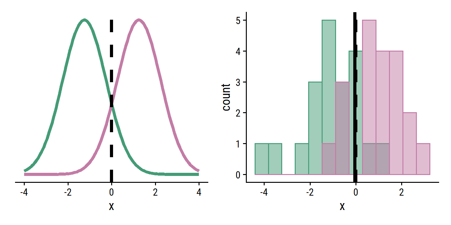

Simulate a large number of test observations and compute the Bayes and LDA test error rates:

set.seed(2021)
d <- tribble(
  ~class, ~x,
  1, rnorm(1e3, mean = mu1, sd = sigma1),
  2, rnorm(1e3, mean = mu2, sd = sigma2)
) %>%
  unnest(x)
# The LDA boundary must be recomputed with the new data
lda_boundary <-
  (mean(filter(d, class == 1)$x) + mean(filter(d, class == 2)$x)) / 2

d %>%
  mutate(
    bayes_class = ifelse(x > bayes_boundary, 1, 2),
    lda_class = ifelse(x > lda_boundary, 1, 2)
  ) %>%
  summarise(
    `Bayes error rate` = mean(class == bayes_class),
    `LDA error rate` = mean(class == lda_class)
  )

## # A tibble: 1 × 2
##   `Bayes error rate` `LDA error rate`
##                <dbl>            <dbl>
## 1              0.104            0.107

Pretty close but, as expected, the Bayes classifier has the lower error rate.

To reiterate, the LDA classifier results from assuming that the observations within each class come from a normal distribution with a class-specific mean and a common variance \(\sigma^2\), and plugging estimates for these parameters into the Bayes classifier. In Section 4.4.3, we will consider a less stringent set of assumptions, by allowing the observations in the \(k\)th class to have a class-specific variance, \(\sigma_k^2\).

4.4.2 Linear Discriminant Analysis for \(p > 1\)

Extending the LDA classifier for multiple predictors involves a multi-variate Gaussian distribution with class-specific mean vector and a common covariance matrix.

The multivariate Gaussian distribution assumes that each individual predictor follows a one-dimensional normal distribution, as in (4.16), with some correlation between each pair of predictors.

I’ll simulate some data with the mvtnorm package and plot probabilities with a 2D density plot (instead of the 3D in Figure 4.5):

d <- crossing(x1 = seq(-2, 2, 0.1), x2 = seq(-2, 2, 0.1))
d1 <- d %>%
  bind_cols(
    prob = mvtnorm::dmvnorm(
      x = as.matrix(d),
      mean = c(0, 0), sigma = matrix(c(1, 0, 0, 1), nrow = 2)
    )
  )
d2 <- d %>%
  bind_cols(
    prob = mvtnorm::dmvnorm(
      x = as.matrix(d),
      mean = c(0, 0), sigma = matrix(c(1, 0.7, 0.7, 1), nrow = 2)
    )
  )
p1 <- d1 %>%
  ggplot(aes(x = x1, y = x2)) +
  geom_tile(aes(fill = prob)) +
  scale_x_continuous(expand = c(0, 0)) +
  scale_y_continuous(expand = c(0, 0)) +
  theme(legend.position = "none")
p2 <- d2 %>%
  ggplot(aes(x = x1, y = x2)) +
  geom_tile(aes(fill = prob)) +
  scale_x_continuous(expand = c(0, 0)) +
  scale_y_continuous(expand = c(0, 0)) +
  theme(legend.position = "none")
p1 | p2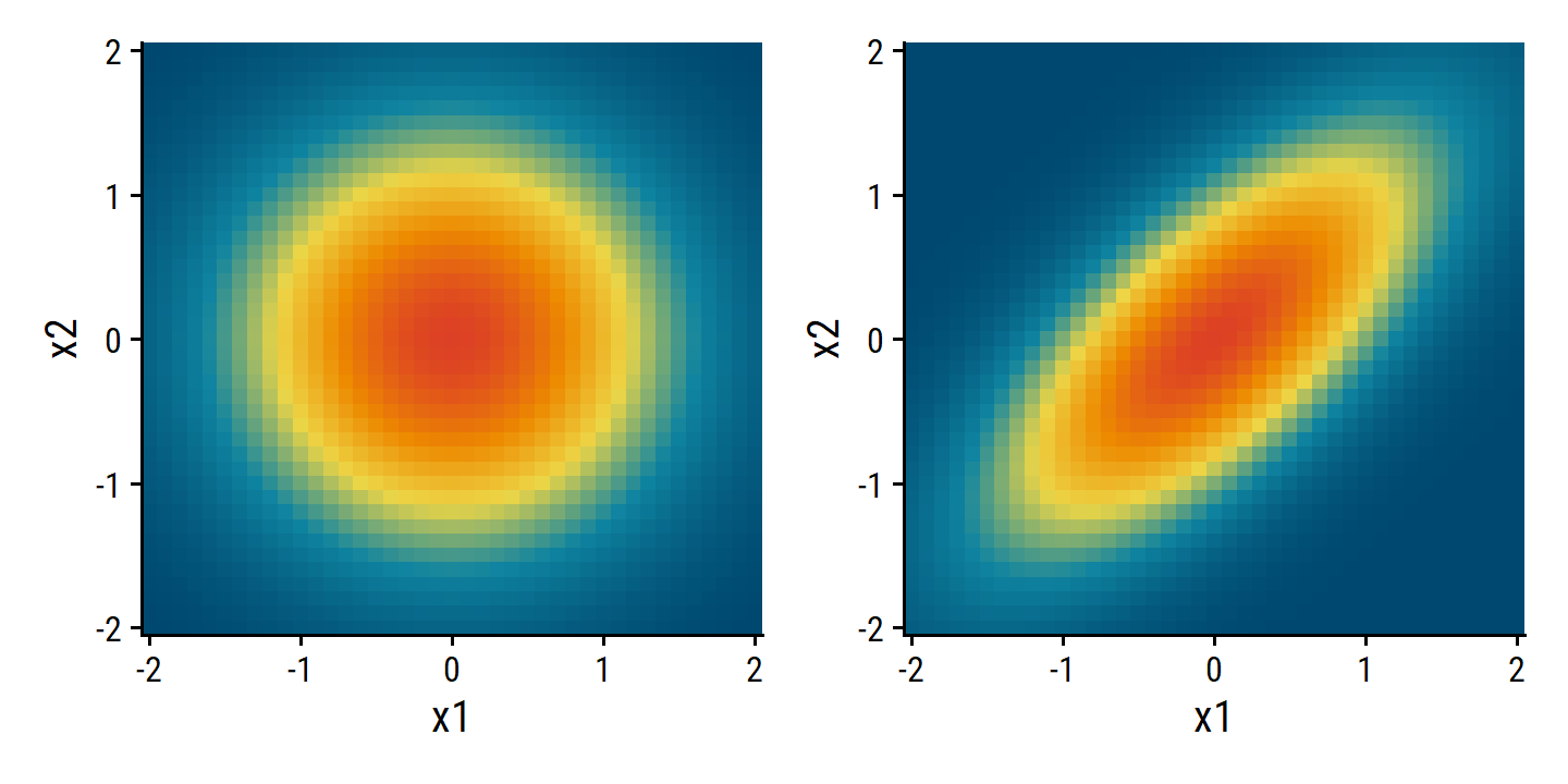

To indicate that a \(p\)-dimensional random variable \(X\) has a multivariate Gaussian distribution, we write \(X \sim N(\mu, \Sigma)\). Here \(E(X) = \mu\) is the mean of \(X\) (a vector with \(p\) components), and \(\text{Cov}(X) = \Sigma\) is the \(p \times p\) covariance matrix of \(X\).

The LDA classifier assumes that the observations in the \(k\)th class are drawn from a multivariate Gaussian distribution \(N(\mu_k, \Sigma)\). The Bayes classifier assigns an observation \(X = x\) to the class for which

\[ \delta_k (x) = x^T \Sigma^{-1} \mu_k - \frac{1}{2} \mu_k^T \Sigma^{-1} \mu_k + \log \pi_k \]

is largest.

As with the univariable case, the LDA method involves estimating the unknown parameters \(\mu_k\), \(\pi_k\) and \(\Sigma\). Then the quantities \(\hat{\delta}_k (x)\) are calculated and the observations \(X\) are classified into the largest \(\hat{\delta}_k (k)\).

We can perform LDA using the MASS package to predict default from student and balance:

lda_default_balance_student <-
  MASS::lda(default ~ balance + student, data = default)
lda_default_balance_student

## Call:
## lda(default ~ balance + student, data = default)
## 
## Prior probabilities of groups:
##     No    Yes 
## 0.9667 0.0333 
## 
## Group means:
##       balance studentYes
## No   803.9438  0.2914037
## Yes 1747.8217  0.3813814
## 
## Coefficients of linear discriminants:
##                     LD1
## balance     0.002244397
## studentYes -0.249059498

# The MASS package has a `select` function that overwrite `dplyr`,
#  fix that before it becomes a problem
select <- dplyr::select

The resulting training error rate:

mean(
  predict(lda_default_balance_student,
          newdata = default)$class != default$default
)

## [1] 0.0275

This sounds like a low error rate, but two caveats must be noted.

• First of all, training error rates will usually be lower than test error rates, which are the real quantity of interest. In other words, we might expect this classifier to perform worse if we use it to predict whether or not a new set of individuals will default. The reason is that we specifically adjust the parameters of our model to do well on the training data. The higher the ratio of parameters \(p\) to number of samples \(n\), the more we expect this overfitting to play a role. For these data we don’t expect this to be a problem, since \(p = 2\) and \(n = 10,000\).
• Second, since only 3.33% of the individuals in the training sample defaulted, a simple but useless classifier that always predicts that an individual will not default, regardless of his or her credit card balance and student status, will result in an error rate of 3.33%. In other words, the trivial null classifier will achieve an error rate that is only a bit higher than the LDA training set error rate.

Make predictions and produce the confusion matrix in Table 4.4:

lda_pred <- 
  bind_cols(
    pred_default = predict(lda_default_balance_student,
                           newdata = default)$class,
    default 
  ) 
lda_pred %>%
  count(pred_default, default) %>%
  pivot_wider(names_from = default, values_from = n) %>%
  mutate(Total = No + Yes) %>%
  gt(rowname_col = "pred_default") %>%
  gt::tab_spanner(label = "True default status", columns = everything()) %>%
  gt::tab_stubhead("Predicted") %>%
  # Can't get the Total row to round to 0 decimals
  gt::summary_rows(fns = list(Total = ~round(sum(.), 0)))

Predicted	True default status
	No	Yes	Total
No	9644	252	9896
Yes	23	81	104
Total	9,667.00	333.00	10,000.00

We only missed 23 individuals who did not default, out of 9667. This is great, but we did quite poorly in predicting defaulters.

However, of the 333 individuals who defaulted, 252 (or 75.7%) were missed by LDA. So while the overall error rate is low, the error rate among individuals who defaulted is very high. From the perspective of a credit card company that is trying to identify high-risk individuals, an error rate of 252/333 = 75.7% among individuals who default may well be unacceptable.

Class-specific performance is also important in medicine and biology, where the terms sensitivity and specificity characterize the performance of a classifier or screening test. In this case the sensitivity is the percentage of true defaulters that are identified; it equals 24.3%. The specificity is the percentage of non-defaulters that are correctly identified; it equals (1 − 23/9667) = 99.8%.

LDA has poor sensitivity here because it attempts to reduce the total error rate, regardless of class. In the case of a credit card company, it is probably more valuable to correctly identify individuals who will default.

The LDA classifier, like the Bayes classifier to which it approximates, assigns an observation to the default = “Yes” class if

\[ \text{Pr}(\text{default = Yes}| X = x) > 0.5. \]

That is to say, these classifiers have a default threshold of 50% posterior probability. We may lower these probability as needed. To adjust this with the MASS::lda package, we can get the posterior probabilities directly via predict.lda():

lda_posterior <- predict(lda_default_balance_student, newdata = default)$posterior
head(lda_posterior)

##          No         Yes
## 1 0.9968680 0.003131975
## 2 0.9971925 0.002807531
## 3 0.9843970 0.015603046
## 4 0.9987769 0.001223133
## 5 0.9959254 0.004074582
## 6 0.9954627 0.004537289

Then use the threshold of 20% to re-create Table 4.5:

lda_pred_20 <- bind_cols(
  default,
  posterior_prob_default = lda_posterior[,2]
) %>%
  mutate(
    pred_default = ifelse(posterior_prob_default > 0.2, "Yes", "No")
  )
lda_pred_20 %>%
  count(pred_default, default) %>%
  pivot_wider(names_from = default, values_from = n) %>%
  mutate(Total = No + Yes) %>%
  gt(rowname_col = "pred_default") %>%
  tab_spanner(label = "True default status", columns = everything()) %>%
  tab_stubhead("Predicted") %>%
  summary_rows(fns = list(Total = ~round(sum(.), 0)))

Predicted	True default status
	No	Yes	Total
No	9432	138	9570
Yes	235	195	430
Total	9,667.00	333.00	10,000.00

The sensitivity to detect defaulters has improved to 58.8%, but the specificity has dropped 97.5%. The overall error rate has also increased to 3.7%.

But a credit card company may consider this slight increase in the total error rate to be a small price to pay for more accurate identification of individuals who do indeed default.

How can we decide which threshold value is best? Such a decision must be based on domain knowledge, such as detailed information about the costs associated with default.

The receiver operating character (ROC) curve is one way to visualize the trade-off between two types of error for different threshold values. I like the yardstick::roc_curve() function for this purpose:

lda_roc <-
  yardstick::roc_curve(
    lda_pred_20,
    # Specify the class probability and the truth variables
    posterior_prob_default, truth = default,
    # This argument specifies which level of truth (default) is considered
    #  "positive", so it will flip the ROC curve vertically
    event_level = "second"
  )
autoplot(lda_roc)

The area under the curve (AUC) summarizes the overall performance of the classifier:

yardstick::roc_auc(
  lda_pred_20,
  posterior_prob_default, truth = default,
  event_level = "second"
)

## # A tibble: 1 × 3
##   .metric .estimator .estimate
##   <chr>   <chr>          <dbl>
## 1 roc_auc binary         0.950

We get the exact same ROC AUC with logistic regression:

glm_default_balance_student <-
  glm(default ~ balance + student,
      data = default, family = binomial)

glm_pred <- bind_cols(
  default,
  glm_prob_default = predict(
    glm_default_balance_student,
    newdata = default, type = "response"
  )
)
yardstick::roc_auc(
  glm_pred,
  glm_prob_default, truth = default,
  event_level = "second"
)

## # A tibble: 1 × 3
##   .metric .estimator .estimate
##   <chr>   <chr>          <dbl>
## 1 roc_auc binary         0.950

4.4.3 Quadratic Discriminant Analysis

As we have discussed, LDA assumes that the observations within each class are drawn from a multivariate Gaussian distribution with a class-specific mean vector and a covariance matrix that is common to all \(K\) classes. Quadratic discriminant analysis (QDA) provides an alternative approach. Like LDA, the QDA classifier results from assuming that the observations from each class are drawn from a Gaussian distribution, and plugging estimates for the parameters into Bayes’ theorem in order to perform prediction. However, unlike LDA, QDA assumes that each class has its own covariance matrix. That is, it assumes that an observation from the \(k\)th class is of the form \(X \sim N(\mu_k, \Sigma_k)\), where \(\Sigma_k\) is a covariance matrix for the \(k\)th class.

An observation \(X = x\) is assigned to the class for which

\[ \begin{align} \delta_k (x) = - \frac{1}{2} (x - \mu_k)^T \Sigma^{-1}_k (x - \mu_k) - \frac{1}{2} \log |\Sigma_k|+ \log \pi_k. \end{align} \]

is largest. QDA gets its name from how the quantity \(x\) appears as quadratic function in the first term of the above equation.

Why does it matter whether or not we assume that the \(K\) classes share a common covariance matrix? In other words, why would one prefer LDA to QDA, or vice-versa? The answer lies in the bias-variance trade-off. When there are \(p\) predictors, then estimating a covariance matrix requires estimating \(p(p+1)/2\) parameters. QDA estimates a separate covariance matrix for each class, for a total of \(Kp(p+1)/2\) parameters.

Consequently, LDA is a much less flexible classifier than QDA, and so has substantially lower variance. This can potentially lead to improved prediction performance. But there is a trade-off: if LDA’s assumption that the \(K\) classes share a common covariance matrix is badly off, then LDA can suffer from high bias.

In general, use LDA if there are relatively few training observations, and use QDA for many. Also consider QDA if you have some intuition about the decision boundary being non-linear.

4.4.4 Naive Bayes

The naive Bayes classifier also estimates the conditional probability \(f_k (x) = \text{Pr}(X|Y = k)\). In LDA, we made the very strong assumption that \(f_k\) is the density function of a multivariate normal distribution with mean \(\mu_k\) and shared covariance \(\Sigma\). In QDA, the covariance \(\Sigma_k\) is class-specific. The naive Bayes classifier instead makes a single assumption:

Within the \(k\)th class, the \(p\) predictors are independent.

Mathematically:

\[ f_k (x) = f_{k1}(x_1) \times f_{k2}(x_2) \times \dots \times f_{kp}(x_p). \]

where \(f_{kj}\) is the density function of the \(j\)th predictor among observations in the \(k\)th class.

Why is this assumption so powerful? Essentially, estimating a \(p\)-dimensional density function is challenging because we must consider not only the marginal distribution of each predictor — that is, the distribution of each predictor on its own — but also the joint distribution of the predictors — that is, the association between the different predictors. In the case of a multivariate normal distribution, the association between the different predictors is summarized by the off-diagonal elements of the covariance matrix. However, in general, this association can be very hard to characterize, and exceedingly challenging to estimate. But by assuming that the \(p\) covariates are independent within each class, we completely eliminate the need to worry about the association between the \(p\) predictors, because we have simply assumed that there is no association between the predictors!

This is a very stringent assumption – most of the time, we believe there to be some degree of association between predictors. But naive Bayes can still perform well, especially when \(n\) is not large enough relative to \(p\) to effectively estimate the joint distribution of the predictors within each class.

Essentially, the naive Bayes assumption introduces some bias, but reduces variance, leading to a classifier that works quite well in practice as a result of the bias-variance trade-off.

Under the naive Bayes, assumption, the posterior probability becomes:

\[ \text{Pr}(Y = k|X = x) = \frac{\pi_k \times f_{k1}(x_1) \times \dots \times f_{kp} (x_p)}{\sum_{l=1}^K \pi_l \times f_{l1}(x_1) \times \dots \times f_{lp} (x_p)} \]

for \(k = 1, \dots, K\).

To estimate the one-dimensional \(f_{kj}\) from \(x_j\), we have a few options:

• Assume that the \(j\)th predictor is drawn from a univariate normal distribution.
  • \(X_j | Y = k \sim N(\mu_{jk}, \sigma_{jk}^2)\).
  • This is like QDA except the covariance matrix is diagonal because the predictors are independent.
• Use a non-parametric estimate for \(f_{kj}\).
  • A simple way: Estimate \(f_{kj}(x_j)\) as the fraction of the training observations in the \(k\)th class belonging to a histogram bin.
  • Alternatively, use a kernel density estimator, which is essentially a smoothed version of a histogram.
• For qualitative \(X_j\), simply count the proportion of training observations for the \(j\)th predictor corresponding to each class.

Apply the naive Bayes classifier with the klaR package:

nb_default <-
  klaR::NaiveBayes(default ~ balance + student, data = default)
nb_pred <- bind_cols(
  default,
  nb_prob_default = predict(nb_default, newdata = default)$posterior[,2]
)

If we take a posterior probability of 50% or 20% as the thresholds for predicting a default, we get Tables 4.8 and 4.9:

nb_pred <- nb_pred %>%
  mutate(
    pred_default_0.5 = ifelse(nb_prob_default > 0.5, "Yes", "No"),
    pred_default_0.2 = ifelse(nb_prob_default > 0.2, "Yes", "No")
  )
nb_pred %>%
  count(pred_default_0.5, default) %>%
  pivot_wider(names_from = default, values_from = n) %>%
  mutate(Total = No + Yes) %>%
  gt(rowname_col = "pred_default_0.5") %>%
  tab_spanner(label = "True default status", columns = everything()) %>%
  tab_stubhead("Predicted") %>%
  summary_rows(fns = list(Total = ~round(sum(.), 0)))

Predicted	True default status
	No	Yes	Total
No	9621	244	9865
Yes	46	89	135
Total	9,667.00	333.00	10,000.00

nb_pred %>%
  count(pred_default_0.2, default) %>%
  pivot_wider(names_from = default, values_from = n) %>%
  mutate(Total = No + Yes) %>%
  gt(rowname_col = "pred_default_0.2") %>%
  tab_spanner(label = "True default status", columns = everything()) %>%
  tab_stubhead("Predicted") %>%
  summary_rows(fns = list(Total = ~round(sum(.), 0)))

Predicted	True default status
	No	Yes	Total
No	9339	130	9469
Yes	328	203	531
Total	9,667.00	333.00	10,000.00

The numbers are slightly different from the text, which may have to do with how \(f_{kj}\) for the quantitative balance was estimated. The overall error rate, sensitivity, and specificity of the naive Bayes approach:

nb_pred %>%
  select(default, pred_default_0.2, pred_default_0.5) %>%
  pivot_longer(c(pred_default_0.5, pred_default_0.2),
               names_to = "threshold", values_to = "pred_default") %>%
  mutate(threshold = as.numeric(str_remove(threshold, "pred_default_"))) %>%
  group_by(threshold) %>%
  summarise(
    overall_error = mean(default != pred_default),
    sensitivity = sum(default == "Yes" & pred_default == "Yes") /
      sum(default == "Yes"),
    specificity = sum(default == "No" & pred_default == "No") /
      sum(default == "No"),
    .groups = "drop"
  ) %>%
  mutate(across(everything(), scales::percent)) %>%
  gt()

threshold	overall_error	sensitivity	specificity
20%	4.6%	61%	96.6%
50%	2.9%	27%	99.5%

The overall error rate is slightly higher, but a higher sensitivity was achieved.

In this example, it should not be too surprising that naive Bayes does not convincingly outperform LDA: this data set has \(n = 10,000\) and \(p = 4\), and so the reduction in variance resulting from the naive Bayes assumption is not necessarily worthwhile. We expect to see a greater pay-off to using naive Bayes relative to LDA or QDA in instances where \(p\) is larger or \(n\) is smaller, so that reducing the variance is very important.

4.5 A Comparison of Classification Methods

4.5.1 An Analytical Comparison

We now perform an analytical (or mathematical) comparison of LDA, QDA, naive Bayes, and logistic regression. We consider these approaches in a setting with \(K\) classes, so that we assign an observation to the class that maximizes \(\text{Pr}(Y = k|X = x)\). Equivalently, we can set \(K\) as the baseline class and assign an observation to the class that maximizes

\[ \log \left(\frac{\text{Pr}(Y = k|X = x)}{\text{Pr}(Y = K |X = x)}\right) \]

for \(k = 1, \dots, K\).

This is the familiar log-odds of class \(k\) compared to baseline class \(K\).

For LDA, we assumed the predictors within each class are drawn from a multivariate normal distribution with shared co-variance matrix. The log-odds can be represented as:

\[ \begin{align} \log \left(\frac{\text{Pr}(Y = k|X = x)}{\text{Pr}(Y = K |X = x)}\right) &= \log \left(\frac{\pi_k f_k(x)}{\pi_K f_K(x)}\right)\\ &= a_k + \sum_{j=1}^p b_{kj} x_j. \end{align} \]

where \(a_k\) and \(b_{kj}\) are functions of \(\pi_k\), \(\mu_k\), and \(\Sigma_k\). Like logistic regression, LDA assumes that the log-odds of the probabilities are linear in \(x\).

Similarly, an additional function \(c_{kjl}\) gives the log-odds in the QDA setting:

\[ \log \left(\frac{\text{Pr}(Y = k|X = x)}{\text{Pr}(Y = K |X = x)}\right) = a_k + \sum_{j=1}^p b_{kj} x_j + \sum_{j=1}^p \sum_{l=1}^p c_{kjl} x_j x_l \]

which is quadratic in \(x\).

Finally, the naive Bayes setting, with one-dimensional \(f_{kj}(x_j)\):

\[ \begin{align} \log \left(\frac{\text{Pr}(Y = k|X = x)}{\text{Pr}(Y = K |X = x)}\right) &= \log \left(\frac{\pi_k f_k(x )}{\pi_K f_K(x)}\right)\\ &= a_k + \sum_{j=1}^p g_{kj} (x_j). \end{align} \]

where \(g_{kj} (x_j) = \log \frac{f_{kj}(x_j)}{f_{Kj} (x_j)}\). This is the form of a generalized additive model, a topic that is discussed further in Chapter 7.

Looking at these forms, we have the following observations:

• LDA is a special case of QDA with \(c_{kjl} = 0\).
• Any classifier with a linear decision boundary is a special case of naive Bayes with \(b_{kj} (x_j) = b_{kj} x_j\). In particular, this means that LDA is a special case of naive Bayes.
• Naive Bayes is also a special case of LDA if \(f_{kj} (x_j)\) is a modeled as a one-dimensional Gaussian distribution.
• QDA and naive Bayes are not special cases of the other.

None of these methods uniformly dominates the others: in any setting, the choice of method will depend on the true distribution of the predictors in each of the \(K\) classes, as well as other considerations, such as the values of \(n\) and \(p\). The latter ties into the bias-variance trade-off.

Then to tie this all to logistic regression, recall the multinomial form:

\[ \log \left( \frac{\text{Pr} (Y = k| X = x)}{\text{Pr} (Y = K| X = x)}\right) = \beta_{k0} + \sum_{j=1}^p \beta_{kj} x_j. \]

This is identical to the linear form of the LDA as both are linear functions of the predictors. The estimation approach differs of course:

In LDA, the coefficients in this linear function are functions of estimates for \(\pi_k\), \(\pi_K\), \(\mu_k\), \(\mu_K\), and \(\Sigma\) obtained by assuming that \(X_1,\dots, X_p\) follow a normal distribution within each class. By contrast, in logistic regression, the coefficients are chosen to maximize the likelihood function (4.5). Thus, we expect LDA to outperform logistic regression when the normality assumption (approximately) holds, and we expect logistic regression to perform better when it does not.

Lastly, some observations about \(K\)-nearest neighbors, which is a non-parametric alternative to classification:

• Because KNN is completely non-parametric, we can expect this approach to dominate LDA and logistic regression when the decision boundary is highly non-linear, provided that \(n\) is very large and \(p\) is small.
• In order to provide accurate classification, KNN requires a lot of observations relative to the number of predictors – that is, \(n\) much larger than \(p\). This has to do with the fact that KNN is non-parametric, and thus tends to reduce the bias while incurring a lot of variance.
• In settings where the decision boundary is non-linear but \(n\) is only modest, or \(p\) is not very small, then QDA may be preferred to KNN. This is because QDA can provide a non-linear decision boundary while taking advantage of a parametric form, which means that it requires a smaller sample size for accurate classification, relative to KNN.
• Unlike logistic regression, KNN does not tell us which predictors are important: we don’t get a table of coefficients as in Table 4.3.

4.5.2 An Empirical Comparison

Without additional simulation details, I can’t exactly re-produce the results of this section, but I’ll attempt it for scenarios 1, 2 and 3 (the linear examples).

There is a function called make_blobs() in the scikit-learn package (documentation here) that I’ve used before to simulate clustered data. From a quick Google search, I found this R package clusteringdatasets which translates the function in R. I adapted the source code to simulate the two-class linear scenarios:

make_blobs <- function(
  n_samples = 40, n_features = 2,
  # By default, class 1 is centered at (0, 0) and class 2 at (1, 1)
  cluster_centers = matrix(c(0, 0, 1, 1), nrow = 2, byrow = TRUE),
  # By default, the two features are uncorrelated with variance = 1
  cluster_covar = matrix(c(1, 0, 0, 1), nrow = 2),
  dist = c("norm", "t"), t_df = 5
) {
  if (ncol(cluster_centers) != n_features) {
    stop("Dimensionality of centers must equal number of features")
  }
  if ((nrow(cluster_covar) != n_features) |
      (ncol(cluster_covar) != n_features)) {
    stop("Dimensionality of covariance matrix must match number of features")
  }
  dist <- match.arg(dist)
  
  # Equally divides each of `n_samples` into the different categories according
  #  to the number of provided classes
  categories <- rep(1:nrow(cluster_centers), length.out = n_samples)
  
  if (dist == "norm") {
    points <- MASS::mvrnorm(n = n_samples, mu = c(0, 0), Sigma = cluster_covar)
  } else if (dist == "t") {
    points <- mvtnorm::rmvt(n = n_samples, delta = c(0, 0), df = t_df,
                            sigma = cluster_covar)
  }
  points <- points + cluster_centers[categories, ]
  
  colnames(points) <- c("x", "y")
  as_tibble(points) %>%
    bind_cols(category = factor(categories))
}

Here is some sample data simulated for the first three scenarios:

set.seed(22)

tribble(
  ~ scenario, ~ data,
  "Scenario 1", make_blobs(n_samples = 40),
  "Scenario 2", make_blobs(n_samples = 40,
                           cluster_covar = matrix(c(1, -0.5, -0.5, 1),
                                                  nrow = 2)),
  "Scenario 3", make_blobs(n_samples = 100,
                           cluster_covar = matrix(c(1, -0.5, -0.5, 1),
                                                  nrow = 2),
                           dist = "t")
) %>%
  unnest(data) %>%
  ggplot(aes(x, y, color = category, shape = category)) +
  geom_point(size = 3) +
  facet_wrap(~ scenario) +
  dunnr::add_facet_borders()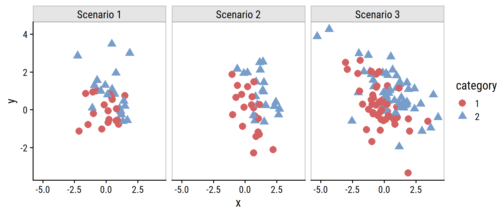

Simulate 100 training data sets for each of these scenarios:

sim_linear_train <- tribble(
  ~ scenario, ~ n_samples, ~ corr, ~ dist,
  "Scenario 1", 40, 0.0, "norm",
  "Scenario 2", 40, -0.5, "norm",
  "Scenario 3", 40, -0.5, "t"
) %>%
  crossing(sim = 1:100) %>%
  rowwise() %>%
  mutate(
    train_data = list(make_blobs(
      n_samples = n_samples,
      cluster_covar = matrix(c(1, corr, corr, 1), nrow = 2),
      dist = dist
    ))
  ) %>%
  ungroup()

The text doesn’t specify how many testing samples are used, just that it is a “large test set.” I’ll use 1000:

sim_linear_test <- sim_linear_train %>%
  distinct(scenario, corr, dist) %>%
  rowwise() %>%
  mutate(
    test_data = list(make_blobs(
      n_samples = 1000,
      cluster_covar = matrix(c(1, corr, corr, 1), nrow = 2),
      dist = dist
    ))
  ) %>%
  ungroup()

Fitting many models to many data sets is made easy with tidymodels, but the code below will be explained more thoroughly later in this book. First, load tidymodels and define the different models to be evaluated:

library(tidymodels)
library(discrim) # this needs to be loaded separately for `discrim_*()`

models <- tribble(
  ~ model_label, ~ model,
  "KNN-1", nearest_neighbor(mode = "classification", neighbors = 1),
  "KNN-CV", nearest_neighbor(mode = "classification", neighbors = tune()),
  "LDA", discrim_linear(),
  "Logistic", logistic_reg(),
  "NBayes", naive_Bayes(engine = "klaR") %>%
    # The klaR engine has an argument usekernel that is always TRUE
    # We have to set it to FALSE to not use KDE, and instead use Gaussian
    #  distributions, as in the text
    set_args(usekernel = FALSE),
  "QDA", discrim_quad()
)

For each model and each of the 100 training sets, fit the model and evaluate on the testing set:

# A helper function for fitting on a training set and getting accuracy from
#  a testing set
calc_test_accuracy <- function(model_label, train_data, test_data, model) {
  wf <- workflow() %>%
    add_recipe(recipe(category ~ x + y, data = train_data)) %>%
    add_model(model)
    
  if (model_label == "KNN-CV") {
    # 5 fold cross-validation
    train_data_folds <- vfold_cv(train_data, v = 5)
    tune_res <- wf %>%
      tune_grid(
        resamples = train_data_folds,
        # Try 1 to 10 neighbors
        grid = tibble(neighbors = 1:10)
      )
    # Overwrite the workflow with the best `neighbors` value by CV accuracy
    wf <- finalize_workflow(wf, select_best(tune_res, "accuracy")) 
  }
  
  wf %>%
    fit(data = train_data) %>%
    augment(test_data) %>%
    accuracy(truth = category, estimate = .pred_class) %>%
    pull(.estimate)
}

tic()
sim_linear_res <-  sim_linear_train %>%
  left_join(sim_linear_test %>% dplyr::select(scenario, test_data),
            by = "scenario") %>%
  crossing(models) %>%
  mutate(
    test_accuracy = pmap_dbl(
      list(model_label, train_data, test_data, model),
      calc_test_accuracy
    ),
    test_error = 1 - test_accuracy
  )
toc()

## 1808.57 sec elapsed

Plot error rate for each model and scenario as in Figure 4.11:

sim_linear_res %>%
  mutate(model_label = fct_inorder(model_label),
         model_fill = fct_collapse(model_label,
                                   KNN = c("KNN-1", "KNN-CV"))) %>%
  ggplot(aes(x = model_label, y = test_error)) +
  geom_boxplot(aes(fill = model_fill), show.legend = FALSE) +
  facet_wrap(~ scenario, nrow = 1, scales = "free_y") +
  dunnr::add_facet_borders() +
  theme(axis.text.x = element_text(angle = 90)) +
  labs(x = NULL, y = "test error")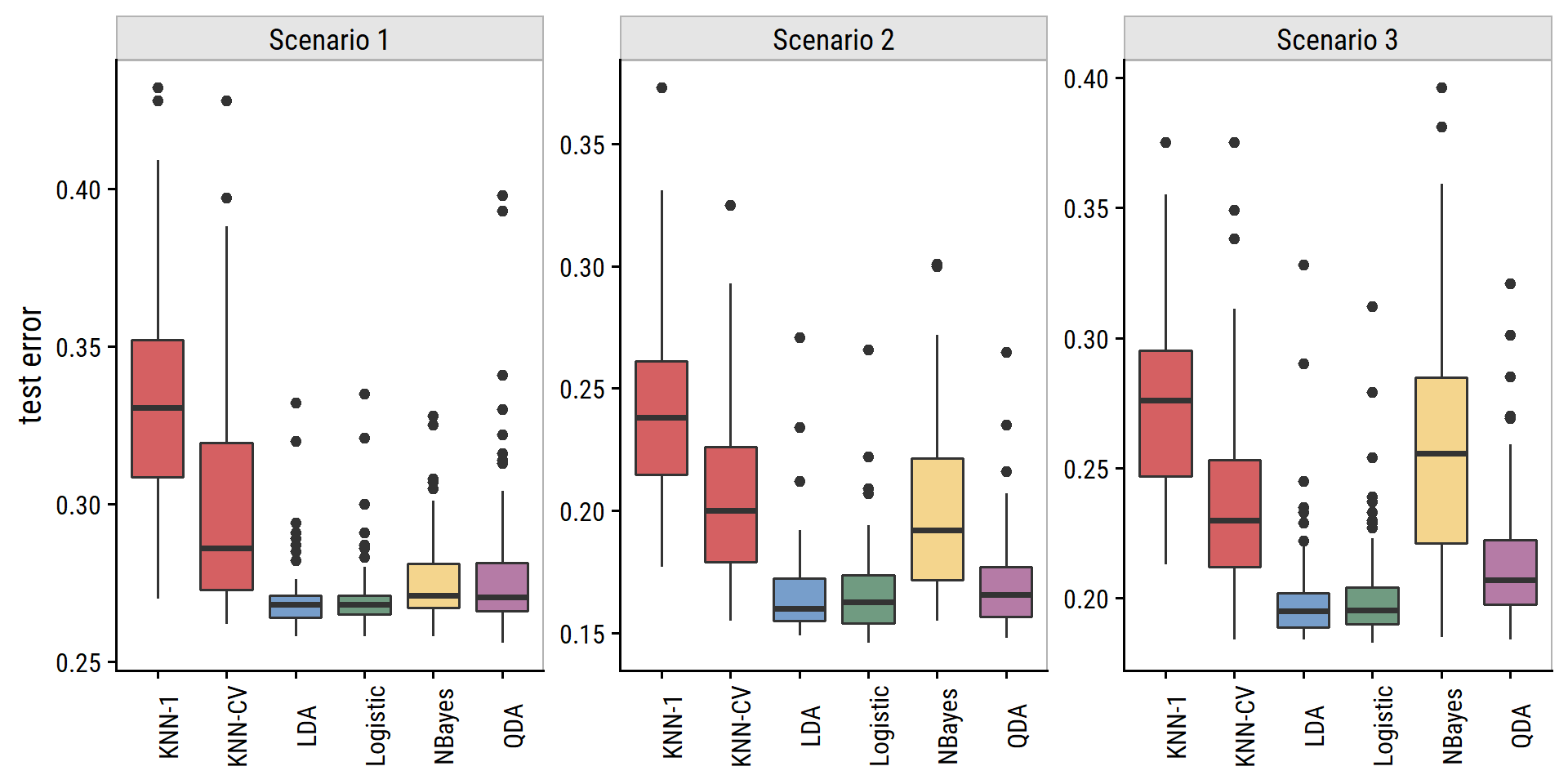

Pretty close.

• Scenario 1: uncorrelated normal variables.
  • LDA and logistic regression performed well due to linear decision boundary.
  • KNN performed poorly.
  • QDA worse than LDA because it was more flexible than necessary.
  • Naive Bayes should be better than QDA because of independent predictors but they are pretty equivalent here.
• Scenario 2: correlated normal variables.
  • Similar to scenario 1, except naive Bayes performed much worse due to correlated predictors.
• Scenario 3: correlated \(t\)-distributed predictors (more extreme points than normal).
  • In the text, logistic regression performs slightly better than LDA, but here they are essentially identical.

I’m not sure of an easy way to adapt this approach to the non-linear scenarios 4, 5 and 6. If anyone reading this has ideas, please share them on this issue. Here is a summary of the results presented in Figure 4.12:

• Scenario 4: normal variables with different correlations per class.
  • The QDA assumption was correct, and therefore greatly outperformed others.
• Scenario 5: uncorrelated normal variables, but responses samples from the logistic function applied to a complicated non-linear function of the predictors.
  • The KNN-CV method gave the best results, followed by the more flexible QDA and naive Bayes.
  • KNN with \(K = 1\) was the worst.
• Scenario 6: normal distribution with a different diagonal covariance matrix (uncorrelated) for each class, and with very small sample size.
  • Naive Bayes performed very well.
  • LDA and logistic regression performed worse due to unequal covariance matrices (non-linear decision boundary).
  • QDA performed a bit worse than naive Bayes due to small sample size, and difficulty estimating correlations between predictors.
  • KNN’s performance also suffered due to very small sample size.

The main takeaway from these empirical examples:

These six examples illustrate that no one method will dominate the others in every situation. When the true decision boundaries are linear, then the LDA and logistic regression approaches will tend to perform well. When the boundaries are moderately non-linear, QDA or naive Bayes may give better results. Finally, for much more complicated decision boundaries, a non-parametric approach such as KNN can be superior. But the level of smoothness for a non-parametric approach must be chosen carefully. In the next chapter we examine a number of approaches for choosing the correct level of smoothness and, in general, for selecting the best overall method.

Finally, recall from Chapter 3 that in the regression setting we can accommodate a non-linear relationship between the predictors and by performing regression using transformations of the predictors. A similar approach could be taken in the classification setting. For instance, we could create a more flexible version of logistic regression by including \(X^2\), \(X^3\), and even \(X^4\) as predictors. This may or may not improve logistic regression’s performance, depending on whether the increase in variance due to the added flexibility is offset by a sufficiently large reduction in bias. We could do the same for LDA. If we added all possible quadratic terms and cross-products to LDA, the form of the model would be the same as the QDA model, although the parameter estimates would be different. This device allows us to move somewhere between an LDA and a QDA model.

4.6 Generalized Linear Models

Thus far, we have considered both quantitative and qualitative response \(Y\). However, sometimes \(Y\) is neither, and so linear regression and classification are not applicable.

The example data set to introduce generalized linear models in bikeshare:

bikeshare <- ISLR2::Bikeshare
glimpse(bikeshare)

## Rows: 8,645
## Columns: 15
## $ season     <dbl> 1, 1, 1, 1, 1, 1, 1, 1, 1, 1, 1, 1, 1, 1, 1, 1, 1, 1, 1, 1,…
## $ mnth       <fct> Jan, Jan, Jan, Jan, Jan, Jan, Jan, Jan, Jan, Jan, Jan, Jan,…
## $ day        <dbl> 1, 1, 1, 1, 1, 1, 1, 1, 1, 1, 1, 1, 1, 1, 1, 1, 1, 1, 1, 1,…
## $ hr         <fct> 0, 1, 2, 3, 4, 5, 6, 7, 8, 9, 10, 11, 12, 13, 14, 15, 16, 1…
## $ holiday    <dbl> 0, 0, 0, 0, 0, 0, 0, 0, 0, 0, 0, 0, 0, 0, 0, 0, 0, 0, 0, 0,…
## $ weekday    <dbl> 6, 6, 6, 6, 6, 6, 6, 6, 6, 6, 6, 6, 6, 6, 6, 6, 6, 6, 6, 6,…
## $ workingday <dbl> 0, 0, 0, 0, 0, 0, 0, 0, 0, 0, 0, 0, 0, 0, 0, 0, 0, 0, 0, 0,…
## $ weathersit <fct> clear, clear, clear, clear, clear, cloudy/misty, clear, cle…
## $ temp       <dbl> 0.24, 0.22, 0.22, 0.24, 0.24, 0.24, 0.22, 0.20, 0.24, 0.32,…
## $ atemp      <dbl> 0.2879, 0.2727, 0.2727, 0.2879, 0.2879, 0.2576, 0.2727, 0.2…
## $ hum        <dbl> 0.81, 0.80, 0.80, 0.75, 0.75, 0.75, 0.80, 0.86, 0.75, 0.76,…
## $ windspeed  <dbl> 0.0000, 0.0000, 0.0000, 0.0000, 0.0000, 0.0896, 0.0000, 0.0…
## $ casual     <dbl> 3, 8, 5, 3, 0, 0, 2, 1, 1, 8, 12, 26, 29, 47, 35, 40, 41, 1…
## $ registered <dbl> 13, 32, 27, 10, 1, 1, 0, 2, 7, 6, 24, 30, 55, 47, 71, 70, 5…
## $ bikers     <dbl> 16, 40, 32, 13, 1, 1, 2, 3, 8, 14, 36, 56, 84, 94, 106, 110…

The response is bikers, the number of hourly users of a bike sharing program in Washington, DC. This response value is neither qualitative nor quantitative: instead, it takes on non-negative integer values, or counts. We will consider counts predicting bikers using the covariates mnth (month of the year), hr (hour of the day, from 0 to 23), workingday (an indicator variable that equals 1 if it is neither a weekend nor a holiday), temp (the normalized temperature, in Celsius), and weathersit (a qualitative variable that takes on one of four possible values: clear; misty or cloudy; light rain or light snow; or heavy rain or heavy snow.) In the analyses that follow, we will treat mnth, hr, and weathersit as qualitative variables.

4.6.1 Linear Regression on the Bikeshare Data

Results of linear regression predicting bikers:

lm_bikers <- lm(bikers ~ mnth + hr + workingday + temp + weathersit,
                data = bikeshare)
tidy_custom(lm_bikers, coef_round = 2, se_round = 2, z_round = 2) %>%
  # Exclude mnth and hr due to space constraints
  filter(!str_detect(term, "mnth|hr")) %>%
  gt()

term	coefficient	std.error	z-statistic	p-value
(Intercept)	-68.63	5.31	-12.93	<0.001
workingday	1.27	1.78	0.71	0.477
temp	157.21	10.26	15.32	<0.001
weathersitcloudy/misty	-12.89	1.96	-6.56	<0.001
weathersitlight rain/snow	-66.49	2.97	-22.42	<0.001
weathersitheavy rain/snow	-109.74	76.67	-1.43	0.152

Re-creating Figure 4.13 takes some wrangling to get the appropriate coefficients:

month_coefs <- tidy(lm_bikers) %>%
  filter(str_detect(term, "Intercept|mnth")) %>%
  transmute(
    Month = ifelse(
      # The reference level is January
      term == "(Intercept)", "Jan",
      str_remove(term, "mnth")
    ) %>%
      fct_inorder(),
    Coefficient = ifelse(
      # The coefficient for the reference level of just the intercept
      term == "(Intercept)", estimate,
      # Otherwise the coefficient is relative to the intercept
      estimate + estimate[term == "(Intercept)"]
    )
  )
hour_coefs <- tidy(lm_bikers) %>%
  filter(str_detect(term, "Intercept|hr")) %>%
  transmute(
    Hour = ifelse(
      # The reference level is 00 hours (midnight)
      term == "(Intercept)", "0",
      str_remove(term, "hr")
    ) %>%
      as.integer(),
    Coefficient = ifelse(
      # The coefficient for the reference level of just the intercept
      term == "(Intercept)", estimate,
      # Otherwise the coefficient is relative to the intercept
      estimate + estimate[term == "(Intercept)"]
    )
  )
p1 <- month_coefs %>%
  ggplot(aes(x = Month, y = Coefficient)) +
  geom_point(color = td_colors$nice$spanish_blue, size = 3) +
  geom_line(aes(group = 1), color = td_colors$nice$spanish_blue, size = 1) +
  theme(axis.text.x = element_text(angle = 45))
p2 <- hour_coefs %>%
  ggplot(aes(x = Hour, y = Coefficient)) +
  geom_point(color = td_colors$nice$spanish_blue, size = 3) +
  geom_line(aes(group = 1), color = td_colors$nice$spanish_blue, size = 1)
p1 | p2

The coefficients make intuitive sense, but the issues with the linear regression become apparent when we look at the predictions:

library(ggdist) # for the stat_halfeye() plotting function

tibble(
  pred_bikers = predict(lm_bikers, newdata = bikeshare,
                        type = "response")
) %>%
  ggplot(aes(x = pred_bikers, fill = stat(x < 0))) +
  stat_halfeye() +
  scale_fill_manual(values = c("grey75", td_colors$nice$ruby_red)) +
  remove_axis("y") +
  theme(legend.position = "none")

9.6% of predictions are negative.

Another problem is heteroskedasticity, as shown in the left of Figure 4.14:

p1 <- bikeshare %>%
  mutate(hr = as.integer(hr)) %>%
  ggplot(aes(x = hr, y = bikers)) +
  geom_jitter(width = 0.1, height = 0, size = 0.5,
              color = td_colors$nice$spanish_blue) +
  # Draw a smoothling spline
  geom_smooth(method = lm, formula = y ~ splines::bs(x, 3), se = FALSE,
              size = 1.5, color = td_colors$nice$emerald)
p2 <- bikeshare %>%
  mutate(hr = as.integer(hr)) %>%
  ggplot(aes(x = hr, y = log(bikers))) +
  geom_jitter(width = 0.1, height = 0, size = 0.5,
              color = td_colors$nice$spanish_blue) +
  geom_smooth(method = lm, formula = y ~ splines::bs(x, 3), se = FALSE,
              size = 1.5, color = td_colors$nice$emerald)
p1 | p2

Lastly, the response bikers is integer-valued, whereas the response in a linear model is continuous.

One solution is to transform the response \(Y\). In the above figure, we see that log(bikers) can fix some of the heteroskedasticity, and also avoids negative predictions. This won’t work if there are any values of bikers = 0, however, and leads to challenging interpretation of the coefficients on the log scale.

4.6.2 Poisson Regression on Bikeshare Data

A much more natural approach to count data is Poisson regression. First, the Poisson distribution:

Suppose that a random variable \(Y\) takes on nonnegative integer values, i.e. \(Y \in \{0, 1, 2, \dots\}\). If \(Y\) follows the Poisson distribution, then

\[ \text{Pr}(Y = k) = \frac{e^{−λ}λ^k}{k!} \text{ for } k = 0, 1, 2, \dots \]

Here, \(λ > 0\) is the expected value of \(Y\), i.e. \(E(Y )\). It turns out that \(λ\) also equals the variance of \(Y\), i.e. \(λ = E(Y ) = \text{Var}(Y )\). This means that if \(Y\) follows the Poisson distribution, then the larger the mean of \(Y\), the larger its variance. (In (4.35), the notation \(k!\), pronounced “k factorial”, is defined as \(k! = k × (k − 1) × (k − 2) × ... × 3 × 2 × 1.\))

As an example, consider biker counts drawn from a Poisson distribution with mean \(E(Y) = \lambda = 5\). Then the probability of 0, 1, 2, etc. bikers during a particular hour is:

tibble(
  n_bikers = 0:6,
  prob = exp(-5) * 5^n_bikers / factorial(n_bikers)
) %>%
  mutate(
    prob = scales::percent(prob)
  )

## # A tibble: 7 × 2
##   n_bikers prob  
##      <int> <chr> 
## 1        0 0.67% 
## 2        1 3.37% 
## 3        2 8.42% 
## 4        3 14.04%
## 5        4 17.55%
## 6        5 17.55%
## 7        6 14.62%

Of course, we expect \(\lambda = E(Y)\) to vary under certain conditions, so we write it as a function of the covariates:

\[ \log (\lambda (X_1, \dots, X_p)) = \beta_0 + \beta_1 X_1 + \dots + \beta_p X_p. \]

Taking the log of \(\lambda\) ensures that \(\lambda(X_1, \dots, X_p)\) takes on non-negative values for all values of the covariates.

The coefficients \(\beta_j\) are estimated using the same maximum likelihood approach as logistic regression:

\[ \ell (\beta_0, \dots, \beta_p) = \prod_{i = 1}^n p(y_i) = \prod_{i = 1}^n \frac{e^{-\lambda (x_i)} \lambda(x_i)^{y_i}}{y_i!} \]

where \(\lambda(x_i) = e^{\beta_0 + \dots + \beta_p x_{i}}\).

Fit the Poisson model:

glm_bikers <- glm(bikers ~ mnth + hr + workingday + temp + weathersit,
                  data = bikeshare, family = poisson)
tidy_custom(glm_bikers, coef_round = 2, se_round = 2, z_round = 2) %>%
  # Exclude mnth and hr due to space constraints
  filter(!str_detect(term, "mnth|hr")) %>%
  gt()

term	coefficient	std.error	z-statistic	p-value
(Intercept)	2.69	0.01	277.12	<0.001
workingday	0.01	0.00	7.50	<0.001
temp	0.79	0.01	68.43	<0.001
weathersitcloudy/misty	-0.08	0.00	-34.53	<0.001
weathersitlight rain/snow	-0.58	0.00	-141.90	<0.001
weathersitheavy rain/snow	-0.93	0.17	-5.55	<0.001

month_coefs <- tidy(glm_bikers) %>%
  filter(str_detect(term, "Intercept|mnth")) %>%
  transmute(
    Month = ifelse(
      term == "(Intercept)", "Jan",
      str_remove(term, "mnth")
    ) %>%
      fct_inorder(),
    Coefficient = ifelse(
      term == "(Intercept)", estimate,
      estimate + estimate[term == "(Intercept)"]
    )
  )
hour_coefs <- tidy(glm_bikers) %>%
  filter(str_detect(term, "Intercept|hr")) %>%
  transmute(
    Hour = ifelse(
      term == "(Intercept)", "0",
      str_remove(term, "hr")
    ) %>%
      as.integer(),
    Coefficient = ifelse(
      term == "(Intercept)", estimate,
      estimate + estimate[term == "(Intercept)"]
    )
  )
p1 <- month_coefs %>%
  ggplot(aes(x = Month, y = Coefficient)) +
  geom_point(color = td_colors$nice$spanish_blue, size = 3) +
  geom_line(aes(group = 1), color = td_colors$nice$spanish_blue, size = 1) +
  theme(axis.text.x = element_text(angle = 45))
p2 <- hour_coefs %>%
  ggplot(aes(x = Hour, y = Coefficient)) +
  geom_point(color = td_colors$nice$spanish_blue, size = 3) +
  geom_line(aes(group = 1), color = td_colors$nice$spanish_blue, size = 1)
p1 | p2

Considerations of this model:

• Qualitatively quite similar to the linear regression model. One difference is that workingday was statistically significant with Poisson regression.
• A coefficient \(\beta_j\) is interpreted as the associated change in \(E(Y) = \lambda\) by a factor of \(\exp({\beta_j})\) for a one unit increase in \(X_j\).
  • Example: a change in weather from clear to cloudy skies is associated with a change of exp(-0.075) = 0.928 = 93% as many people will use bikes.
• The key assumption of the Poisson model is that the variance increases with the mean, \(\lambda = E(Y) = \text{Var}(Y)\), which means it can deal with the heteroskedasticity we saw in the linear model.
• The predictions from the Poisson model, by construction, are non-negative:

tibble(
  pred_bikers = predict(glm_bikers, newdata = bikeshare,
                        type = "response")
) %>%
  ggplot(aes(x = pred_bikers, fill = stat(x < 0))) +
  stat_halfeye() +
  scale_fill_manual(values = c("grey75", td_colors$nice$ruby_red)) +
  remove_axis("y") +
  theme(legend.position = "none")

4.6.3 Generalized Linear Models in Greater Generality

The three regression models we have seen so far (linear, logistic and Poisson) share these similarities.

• Predictors \(X_1, \dots, X_p\) used to predict a response \(Y\), which we assume belongs to a certain family of distributions conditional on \(X\).
  • For linear regression, we typically assume Gaussian/normal.
  • For logistic regression, we assume a Bernoulli distribution.
  • For Poisson regression, we assume a Poisson distribution.
• The mean of \(Y\) is modeled as a function of the predictors:

\[ \begin{align} E(Y|X) &= \beta_0 + \beta_1 X_1 + \dots + \beta_p X_p \\ E(Y|X) &= \frac{e^{\beta_0 + \dots + \beta_pX_p}}{1 + e^{\beta_0 + \dots + \beta_pX_p}} \\ E(Y|X) = \lambda (X_1, \dots, X_p) &= e^{\beta_0 + \beta_1 X_1 + \dots + \beta_p X_p}. \end{align} \]

These three equations can be expressed using a link function \(\eta\), which applies a transformation to \(E(Y|X)\) so that the transformed mean is a lienar function of the predictors:

\[ \eta(E(Y|X)) = \beta_0 + \beta_1 X_1 + \dots + \beta_p X_p. \]

The link functions for linear, logistic, and Poisson regression are, respectively:

\[ \begin{align} \eta(\mu) &= \mu \\ \eta(\mu) &= \log \left(\frac{\mu}{1 - \mu} \right) \\ \eta(\mu) &= \log (\mu). \end{align} \]

The Gaussian, Bernoulli, and Poisson distributions are all members of a wider class of distributions, known as the exponential family. Other well-known members of this family are the exponential distribution, the Gamma distribution, and the negative binomial distribution. In general, we can perform a regression by modeling the response \(Y\) as coming from a particular member of the exponential family, and then transforming the mean of the response so that the transformed mean is a linear function of the predictors via (4.42). Any regression approach that follows this very general recipe is known as a generalized linear model (GLM). Thus, linear regression, logistic regression, and Poisson regression and three examples of GLMs. Other examples not covered here include Gamma regression and negative binomial regerssion.

4.7 Lab: Classification Methods

4.7.1 The Stock Market Data

We will begin by examining some numerical and graphical summaries of the Smarket data, which is part of the ISLR2 library. This data set consists of percentage returns for the S&P 500 stock index over 1,250 days, from the beginning of 2001 until the end of 2005. For each date, we have recorded the percentage returns for each of the five previous trading days, Lag1 through Lag5. We have also recorded Volume (the number of shares traded on the previous day, in billions), Today (the percentage return on the date in question) and Direction (whether the market was Up or Down on this date). Our goal is to predict Direction (a qualitative response) using the other features.

I like the skimr package for summarizing a data set:

smarket <- ISLR2::Smarket
skimr::skim(smarket)

Table 4.1: Data summary

Name	smarket
Number of rows	1250
Number of columns	9
_______________________
Column type frequency:
factor	1
numeric	8
________________________
Group variables	None

Variable type: factor

skim_variable	n_missing	complete_rate	ordered	n_unique	top_counts
Direction	0	1	FALSE	2	Up: 648, Dow: 602

Variable type: numeric

skim_variable	n_missing	complete_rate	mean	sd	p0	p25	p50	p75	p100	hist
Year	0	1	2003.02	1.41	2001.00	2002.00	2003.00	2004.00	2005.00	▇▇▇▇▇
Lag1	0	1	0.00	1.14	-4.92	-0.64	0.04	0.60	5.73	▁▃▇▁▁
Lag2	0	1	0.00	1.14	-4.92	-0.64	0.04	0.60	5.73	▁▃▇▁▁
Lag3	0	1	0.00	1.14	-4.92	-0.64	0.04	0.60	5.73	▁▃▇▁▁
Lag4	0	1	0.00	1.14	-4.92	-0.64	0.04	0.60	5.73	▁▃▇▁▁
Lag5	0	1	0.01	1.15	-4.92	-0.64	0.04	0.60	5.73	▁▃▇▁▁
Volume	0	1	1.48	0.36	0.36	1.26	1.42	1.64	3.15	▁▇▅▁▁
Today	0	1	0.00	1.14	-4.92	-0.64	0.04	0.60	5.73	▁▃▇▁▁

To produce the pairwise correlations between predictors, I’ll use another new package corrr, which returns a tidy tibble that we can turn into a nice gt table:

smarket %>% select(-Direction) %>%
  corrr::correlate(method = "pearson", quiet = TRUE) %>%
  gt(rowname_col = "term") %>%
  gt::fmt_missing(columns = everything(), missing_text = "") %>%
  gt::data_color(
    columns = everything(),
    colors = scales::col_numeric(
      palette = td_pal("div5")(5),
      domain = c(-0.1, 0.6)
    )
  ) %>%
  gt::fmt_number(columns = everything(), decimals = 3)

## Warning: The `fmt_missing()` function is deprecated and will soon be removed
## * Use the `sub_missing()` function instead

	Year	Lag1	Lag2	Lag3	Lag4	Lag5	Volume	Today
Year		0.030	0.031	0.033	0.036	0.030	0.539	0.030
Lag1	0.030		−0.026	−0.011	−0.003	−0.006	0.041	−0.026
Lag2	0.031	−0.026		−0.026	−0.011	−0.004	−0.043	−0.010
Lag3	0.033	−0.011	−0.026		−0.024	−0.019	−0.042	−0.002
Lag4	0.036	−0.003	−0.011	−0.024		−0.027	−0.048	−0.007
Lag5	0.030	−0.006	−0.004	−0.019	−0.027		−0.022	−0.035
Volume	0.539	0.041	−0.043	−0.042	−0.048	−0.022		0.015
Today	0.030	−0.026	−0.010	−0.002	−0.007	−0.035	0.015

The only substantial correlation is between Volume and Year:

smarket %>%
  ggplot(aes(x = factor(Year), y = Volume)) +
  geom_jitter(width = 0.3, color = td_colors$nice$day9_yellow) +
  geom_boxplot(alpha = 0.3, outlier.shape = NA, width = 0.2)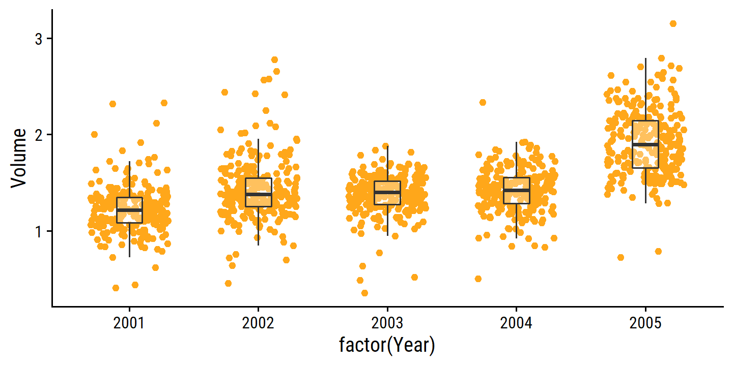

4.7.2 Logistic Regression

Use tidymodels to fit the model and produce the confusion matrix:

glm_direction_fit <-
  # Note that these options are the defaults
  #  (and mode can only be "classification" for logistic)
  logistic_reg(mode = "classification", engine = "glm") %>%
  fit(Direction ~ Lag1 + Lag2 + Lag3 + Lag4 + Lag5 + Volume,
      data = smarket)

glm_direction_conf_mat <-
  augment(glm_direction_fit, smarket) %>%
  yardstick::conf_mat(.pred_class, Direction)
glm_direction_conf_mat

##           Truth
## Prediction Down  Up
##       Down  145 457
##       Up    141 507

This returns an object with some helpful built-in functions. Summary metrics:

summary(glm_direction_conf_mat)

## # A tibble: 13 × 3
##    .metric              .estimator .estimate
##    <chr>                <chr>          <dbl>
##  1 accuracy             binary        0.522 
##  2 kap                  binary        0.0237
##  3 sens                 binary        0.507 
##  4 spec                 binary        0.526 
##  5 ppv                  binary        0.241 
##  6 npv                  binary        0.782 
##  7 mcc                  binary        0.0277
##  8 j_index              binary        0.0329
##  9 bal_accuracy         binary        0.516 
## 10 detection_prevalence binary        0.482 
## 11 precision            binary        0.241 
## 12 recall               binary        0.507 
## 13 f_meas               binary        0.327

We get the same accuracy (52.2%) as that in the text. There is also a couple autoplot() options

autoplot(glm_direction_conf_mat, type = "mosaic") |
  autoplot(glm_direction_conf_mat, type = "heatmap")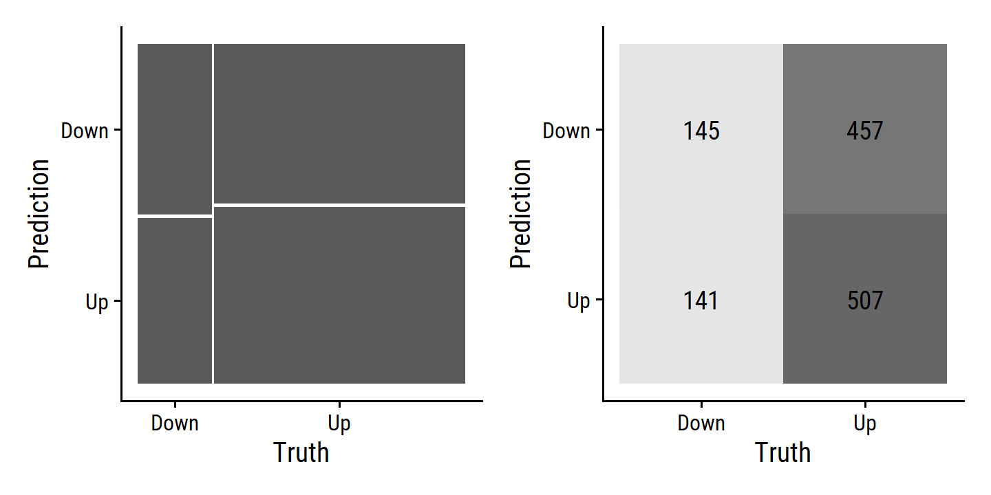

The next part of this lab is (I think) the first time we are splitting the data into training and testing data. Typically in tidymodels, we randomly split the data with rsample::initial_split, which takes a specified proportion (prop) and optional stratification variable (strata). In this lab, all the data for Year = 2005 is the hold out set. We can re-create this split manually with rsample::make_splits:

smarket_split <-
  make_splits(
    x = list(
      # Get row numbers for <2005
      "analysis" = which(smarket$Year < 2005),
      # Get row numbers for 2005
      "assessment" = which(smarket$Year == 2005)
    ),
    data = smarket
  )
smarket_split

## <Analysis/Assess/Total>
## <998/252/1250>

We then get the training and testing data with their matching functions:

smarket_train <- training(smarket_split)
smarket_test <- testing(smarket_split)

Re-fit the model using the training data only:

glm_direction_fit <-
  logistic_reg(mode = "classification", engine = "glm") %>%
  fit(Direction ~ Lag1 + Lag2 + Lag3 + Lag4 + Lag5 + Volume,
      data = smarket_train)

Just as a demonstration, I will evaluate the model on the training data first:

glm_direction_train_pred <-
  glm_direction_fit %>%
  augment(smarket_train)
glm_direction_train_pred %>%
  accuracy(truth = Direction, .pred_class)

## # A tibble: 1 × 3
##   .metric  .estimator .estimate
##   <chr>    <chr>          <dbl>
## 1 accuracy binary         0.527

Quite poor. This was calculated using the 50% probability threshold, but we can also look at the ROC curve:

glm_direction_train_pred %>%
  roc_curve(truth = Direction, .pred_Up,
            event_level = "second") %>%
  autoplot()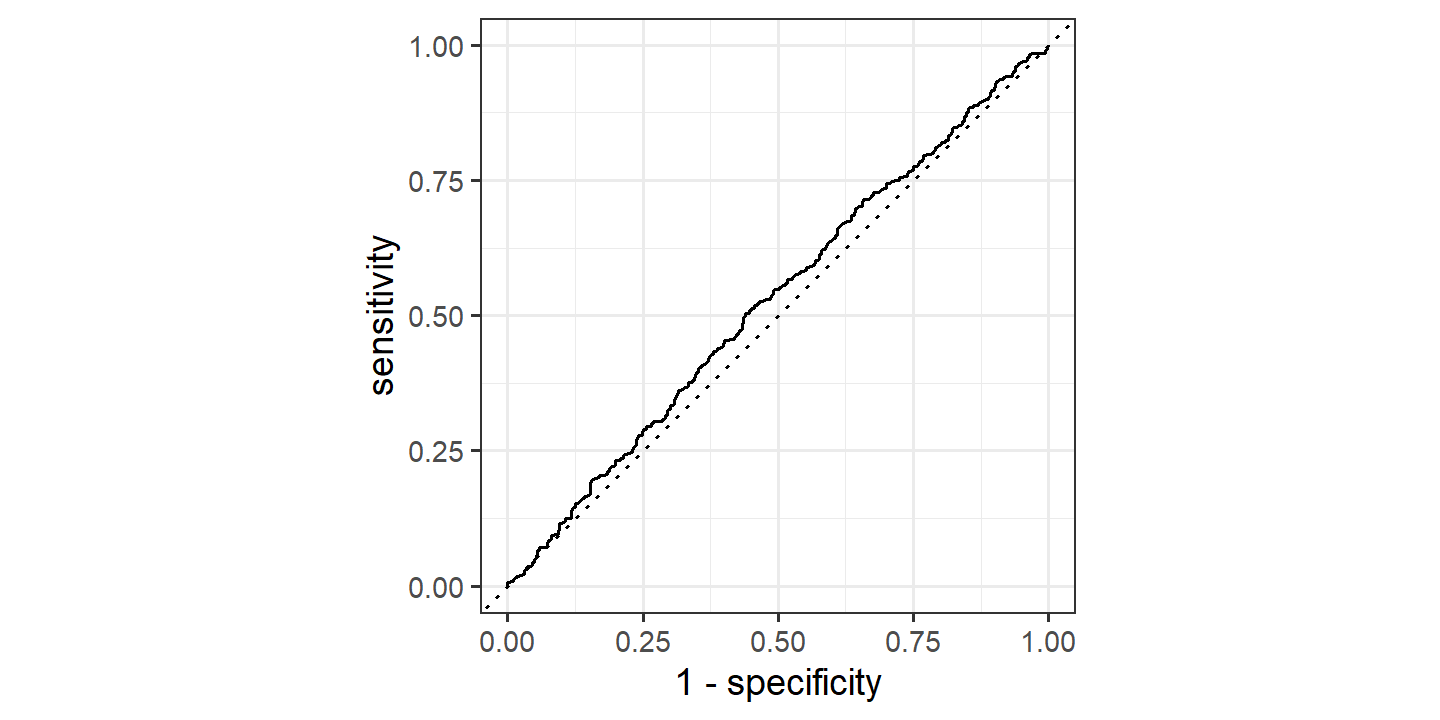

This doesn’t give a lot of confidence in the performance on the testing set:

glm_direction_test_pred <-
  glm_direction_fit %>%
  augment(smarket_test)
glm_direction_test_pred %>%
  accuracy(truth = Direction, .pred_class)

## # A tibble: 1 × 3
##   .metric  .estimator .estimate
##   <chr>    <chr>          <dbl>
## 1 accuracy binary         0.480

We get an accuracy that is worse than random guessing. Disappointing, but not a surprise as the authors say:

Of course this result is not all that surprising, given that one would not generally expect to be able to use previous days’ returns to predict future market performance. (After all, if it were possible to do so, then the authors of this book would be out striking it rich rather than writing a statistics textbook.)

Perhaps a simpler model would be more effective.

After all, using predictors that have no relationship with the response tends to cause a deterioration in the test error rate (since such predictors cause an increase in variance without a corresponding decrease in bias), and so removing such predictors may in turn yield an improvement.

glm_direction_fit_simple <-
  logistic_reg(mode = "classification", engine = "glm") %>%
  fit(Direction ~ Lag1 + Lag2,
      data = smarket_train)
glm_direction_fit_simple %>%
  augment(smarket_test) %>%
  accuracy(truth = Direction, .pred_class)

## # A tibble: 1 × 3
##   .metric  .estimator .estimate
##   <chr>    <chr>          <dbl>
## 1 accuracy binary         0.560

Indeed it does.

4.7.3 Linear Discriminant Analysis

Perform LDA to predict Direction from Lag1 and Lag2:

library(discrim)
lda_direction_fit <-
  # Note that this model definition does not come with parsnip, but the
  #  extension package discrim
  discrim_linear(mode = "classification", engine = "MASS") %>%
  fit(Direction ~ Lag1 + Lag2, data = smarket_train)
lda_direction_fit

## parsnip model object
## 
## Call:
## lda(Direction ~ Lag1 + Lag2, data = data)
## 
## Prior probabilities of groups:
##     Down       Up 
## 0.491984 0.508016 
## 
## Group means:
##             Lag1        Lag2
## Down  0.04279022  0.03389409
## Up   -0.03954635 -0.03132544
## 
## Coefficients of linear discriminants:
##             LD1
## Lag1 -0.6420190
## Lag2 -0.5135293

Performance on the testing data set:

lda_direction_test_pred <-
  lda_direction_fit %>%
  augment(new_data = smarket_test)
lda_direction_test_pred %>%
  conf_mat(truth = Direction, estimate = .pred_class)

##           Truth
## Prediction Down  Up
##       Down   35  35
##       Up     76 106

lda_direction_test_pred %>%
  accuracy(truth = Direction, estimate = .pred_class)

## # A tibble: 1 × 3
##   .metric  .estimator .estimate
##   <chr>    <chr>          <dbl>
## 1 accuracy binary         0.560

Though there is a package called probably for adjusting probability thresholds for classification metrics, I will just manually do so here:

lda_direction_test_pred %>%
  filter(.pred_Down > 0.9)

## # A tibble: 0 × 12
## # … with 12 variables: Year <dbl>, Lag1 <dbl>, Lag2 <dbl>, Lag3 <dbl>,
## #   Lag4 <dbl>, Lag5 <dbl>, Volume <dbl>, Today <dbl>, Direction <fct>,
## #   .pred_class <fct>, .pred_Down <dbl>, .pred_Up <dbl>
## # ℹ Use `colnames()` to see all variable names

max(lda_direction_test_pred$.pred_Down)

## [1] 0.520235

4.7.4 Quadratic Discriminant Analysis

Performing QDA will look very similar:

qda_direction_fit <-
  discrim_quad(mode = "classification", engine = "MASS") %>%
  fit(Direction ~ Lag1 + Lag2, data = smarket_train)
qda_direction_fit

## parsnip model object
## 
## Call:
## qda(Direction ~ Lag1 + Lag2, data = data)
## 
## Prior probabilities of groups:
##     Down       Up 
## 0.491984 0.508016 
## 
## Group means:
##             Lag1        Lag2
## Down  0.04279022  0.03389409
## Up   -0.03954635 -0.03132544

qda_direction_test_pred <-
  qda_direction_fit %>%
  augment(new_data = smarket_test)
qda_direction_test_pred %>%
  conf_mat(truth = Direction, estimate = .pred_class)

##           Truth
## Prediction Down  Up
##       Down   30  20
##       Up     81 121

qda_direction_test_pred %>%
  accuracy(truth = Direction, estimate = .pred_class)

## # A tibble: 1 × 3
##   .metric  .estimator .estimate
##   <chr>    <chr>          <dbl>
## 1 accuracy binary         0.599

This level of accuracy is quite impressive for stock market data, suggesting that the quadratic form may capture the true relationship more accurately.

4.7.5 Naive Bayes

By default, the discrim::naive_Bayes() function uses the klaR package as the engine (e1071 is not an option).

nb_direction_fit <-
  naive_Bayes(mode = "classification", engine = "klaR") %>%
  # The klaR engine has an argument usekernel that is always TRUE
  # We have to set it to FALSE to not use KDE, and instead use Gaussian
  #  distributions, as in the text
  set_args(usekernel = FALSE) %>%
  fit(Direction ~ Lag1 + Lag2, data = smarket_train)
# The model output is quite long, so I won't print it here
# nb_direction_fit

nb_direction_test_pred <-
  nb_direction_fit %>%
  augment(new_data = smarket_test)
nb_direction_test_pred %>%
  conf_mat(truth = Direction, estimate = .pred_class)

##           Truth
## Prediction Down  Up
##       Down   28  20
##       Up     83 121

nb_direction_test_pred %>%
  accuracy(truth = Direction, estimate = .pred_class)

## # A tibble: 1 × 3
##   .metric  .estimator .estimate
##   <chr>    <chr>          <dbl>
## 1 accuracy binary         0.591

The naive Bayes approach was quite close (a bit worse) than QDA. This makes sense. As we saw in the correlation matrix, the Lag1 and Lag2 are uncorrelated, so the assumption of naive Bayes is not violated.

4.7.6 \(K\)-Nearest Neighbors

I’ll skip right to the \(K = 3\) neighbors fit:

knn_direction_fit <-
  nearest_neighbor(mode = "classification", engine = "kknn",
                   neighbors = 3) %>%
  fit(Direction ~ Lag1 + Lag2, data = smarket_train)

knn_direction_test_pred <-
  knn_direction_fit %>%
  augment(new_data = smarket_test)
knn_direction_test_pred %>%
  conf_mat(truth = Direction, estimate = .pred_class)

##           Truth
## Prediction Down Up
##       Down   43 58
##       Up     68 83

knn_direction_test_pred %>%
  accuracy(truth = Direction, estimate = .pred_class)

## # A tibble: 1 × 3
##   .metric  .estimator .estimate
##   <chr>    <chr>          <dbl>
## 1 accuracy binary           0.5

Essentially a coin flip.

To show a case where KNN does perform well, load the Caravan data set:

caravan <- ISLR2::Caravan

This data set includes a massive 85 predictors that measure demographics for 5822 individuals who did or did not Purchase a caravan insurance policy.

caravan %>% count(Purchase) %>% mutate(p = n / sum(n))

##   Purchase    n          p
## 1       No 5474 0.94022673
## 2      Yes  348 0.05977327

Split the data into training and testing based on row number:

caravan_split <-
  make_splits(
    x = list("assessment" = 1:1000,
               "analysis" = 1001:nrow(caravan)),
    data = caravan
  )
caravan_split

## <Analysis/Assess/Total>
## <4822/1000/5822>

caravan_train <- training(caravan_split)
caravan_test <- testing(caravan_split)

KNN predicts a class based on nearby observations, and so the scale of the variables matters.

For instance, imagine a data set that contains two variables, salary and age (measured in dollars and years, respectively). As far as KNN is concerned, a difference of $1,000 in salary is enormous compared to a difference of 50 years in age. Consequently, salary will drive the KNN classification results, and age will have almost no effect. This is contrary to our intuition that a salary difference of $1,000 is quite small compared to an age difference of 50 years.

To deal with this, we standardize/normalize the data to have mean zero and standard deviation one. In tidymodels, this means we define a recipe with the step_normalize() step:

caravan_rec <- recipe(Purchase ~ ., data = caravan_train) %>%
  step_normalize(all_numeric_predictors())

Then we define the models with 1, 3, and 5 neighbors:

knn_spec1 <-
  nearest_neighbor(mode = "classification", engine = "kknn", neighbors = 1)
knn_spec3 <-
  nearest_neighbor(mode = "classification", engine = "kknn", neighbors = 3)
knn_spec5 <-
  nearest_neighbor(mode = "classification", engine = "kknn", neighbors = 5)

We put the model and recipe together into three separate workflows:

knn_purchase_wf1 <- workflow() %>%
  add_recipe(caravan_rec) %>%
  add_model(knn_spec1)
knn_purchase_wf3 <- workflow() %>%
  add_recipe(caravan_rec) %>%
  add_model(knn_spec3)
knn_purchase_wf5 <- workflow() %>%
  add_recipe(caravan_rec) %>%
  add_model(knn_spec5)

Fit all the models:

knn_purchase_fit1 <- knn_purchase_wf1 %>%
  fit(caravan_train)
knn_purchase_fit3 <- knn_purchase_wf3 %>%
  fit(caravan_train)
knn_purchase_fit5 <- knn_purchase_wf5 %>%
  fit(caravan_train)

Compile the metrics:

knn_metrics <- metric_set(accuracy, sensitivity, specificity, ppv,)
bind_rows(
  augment(knn_purchase_fit1, new_data = caravan_test) %>%
    knn_metrics(truth = Purchase, estimate = .pred_class) %>%
    mutate(neighbors = 1),
  augment(knn_purchase_fit3, new_data = caravan_test) %>%
    knn_metrics(truth = Purchase, estimate = .pred_class) %>%
    mutate(neighbors = 3),
  augment(knn_purchase_fit5, new_data = caravan_test) %>%
    knn_metrics(truth = Purchase, estimate = .pred_class) %>%
    mutate(neighbors = 5)
) %>%
  transmute(neighbors, .metric, .estimate = round(.estimate, 3)) %>%
  pivot_wider(names_from = .metric, values_from = .estimate) %>%
  gt()

neighbors	accuracy	sensitivity	specificity	ppv
1	0.883	0.929	0.153	0.946
3	0.884	0.930	0.153	0.946
5	0.883	0.929	0.153	0.946

The percentages reported in the text are the positive predictive value (TP / (TP + FP)). This is the ppv variable in the above table, which is way off. This is due to the event_level argument to the ppv() metric function (and sensitivity and specificity for that matter). It is calculated the PPV for the first level of the response, which is Purchase = “No’. Re-calculate PPV with the correct”positive” event identified:

bind_rows(
  augment(knn_purchase_fit1, new_data = caravan_test) %>%
    ppv(truth = Purchase, estimate = .pred_class, event_level = "second") %>%
    mutate(neighbors = 1),
  augment(knn_purchase_fit3, new_data = caravan_test) %>%
    ppv(truth = Purchase, estimate = .pred_class, event_level = "second") %>%
    mutate(neighbors = 3),
  augment(knn_purchase_fit5, new_data = caravan_test) %>%
    ppv(truth = Purchase, estimate = .pred_class, event_level = "second") %>%
    mutate(neighbors = 5)
) %>%
  transmute(neighbors, .metric, .estimate = round(.estimate, 3)) %>%
  pivot_wider(names_from = .metric, values_from = .estimate) %>%
  gt()

neighbors	ppv
1	0.118
3	0.120
5	0.118

I’m not getting the improved PPV with increasing neighbors as in the text. Not sure why.

Lastly, get the PPV from a logistic regression:

glm_purchase_wf <- workflow() %>%
  add_recipe(caravan_rec) %>%
  add_model(logistic_reg())
glm_purchase_fit <- glm_purchase_wf %>%
  fit(caravan_train)

## Warning: glm.fit: fitted probabilities numerically 0 or 1 occurred

PPV with a default 50% threshold:

augment(glm_purchase_fit, new_data = caravan_test) %>%
  ppv(truth = Purchase, estimate = .pred_class, event_level = "second")

## # A tibble: 1 × 3
##   .metric .estimator .estimate
##   <chr>   <chr>          <dbl>
## 1 ppv     binary             0

PPV with a 25% threshold:

augment(glm_purchase_fit, new_data = caravan_test) %>%
  mutate(
    .pred_class = ifelse(.pred_Yes > 0.25, "Yes", "No") %>% factor()
  ) %>%
  ppv(truth = Purchase, estimate = .pred_class, event_level = "second")

## # A tibble: 1 × 3
##   .metric .estimator .estimate
##   <chr>   <chr>          <dbl>
## 1 ppv     binary         0.333

4.7.7 Poisson Regression

We will again fit the bikeshare data with Poisson regression, but this time with tidymodels:

library(poissonreg)
glm_bikers_model <-
  poisson_reg(mode = "regression", engine = "glm")

The model specification for poisson_reg() is a model wrapper that comes from the poissonreg package.

It is good practice to explicitly state that we are making dummy variables of the categorical predictors via step_dummy():

glm_bikers_rec <-
  recipe(bikers ~ mnth + hr + workingday + temp + weathersit,
         data = bikeshare) %>%
  step_dummy(all_nominal_predictors())

Define the workflow and fit the model:

glm_bikers_wf <- workflow() %>%
  add_model(glm_bikers_model) %>%
  add_recipe(glm_bikers_rec)
glm_bikers_fit <- glm_bikers_wf %>%
  fit(bikeshare)

We’ve already re-created Figure 4.15 with this model, so won’t repeat it here. Instead, here is a plot of predictions and, just for fun, it is stratified by the weather:

augment(glm_bikers_fit, new_data = bikeshare) %>%
  ggplot(aes(x = bikers, y = .pred)) +
  geom_point(color = td_colors$nice$opera_mauve, alpha = 0.4) +
  geom_abline(slope = 1, size = 1, lty = 2) +
  facet_wrap(~weathersit) +
  theme(legend.position = "none") +
  add_facet_borders()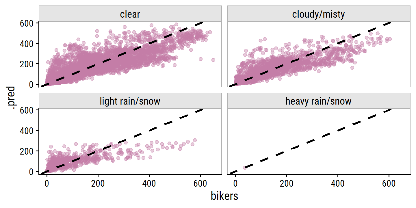

4.8 Exercises

Applied

13. Predict returns with Weekly

weekly <- ISLR2::Weekly

1. Data summaries.

skimr::skim(weekly)

Table 4.2: Data summary

Name	weekly
Number of rows	1089
Number of columns	9
_______________________
Column type frequency:
factor	1
numeric	8
________________________
Group variables	None

Variable type: factor

skim_variable	n_missing	complete_rate	ordered	n_unique	top_counts
Direction	0	1	FALSE	2	Up: 605, Dow: 484

Variable type: numeric

skim_variable	n_missing	complete_rate	mean	sd	p0	p25	p50	p75	p100	hist
Year	0	1	2000.05	6.03	1990.00	1995.00	2000.00	2005.00	2010.00	▇▆▆▆▆
Lag1	0	1	0.15	2.36	-18.20	-1.15	0.24	1.41	12.03	▁▁▆▇▁
Lag2	0	1	0.15	2.36	-18.20	-1.15	0.24	1.41	12.03	▁▁▆▇▁
Lag3	0	1	0.15	2.36	-18.20	-1.16	0.24	1.41	12.03	▁▁▆▇▁
Lag4	0	1	0.15	2.36	-18.20	-1.16	0.24	1.41	12.03	▁▁▆▇▁
Lag5	0	1	0.14	2.36	-18.20	-1.17	0.23	1.41	12.03	▁▁▆▇▁
Volume	0	1	1.57	1.69	0.09	0.33	1.00	2.05	9.33	▇▂▁▁▁
Today	0	1	0.15	2.36	-18.20	-1.15	0.24	1.41	12.03	▁▁▆▇▁

weekly %>% select(-Direction) %>%
  corrr::correlate(method = "pearson", quiet = TRUE) %>%
  gt(rowname_col = "term") %>%
  gt::fmt_missing(columns = everything(), missing_text = "") %>%
  gt::data_color(
    columns = everything(),
    colors = scales::col_numeric(
      palette = td_pal("div5")(5),
      domain = c(-0.1, 0.9)
    )
  ) %>%
  gt::fmt_number(columns = everything(), decimals = 3)

## Warning: The `fmt_missing()` function is deprecated and will soon be removed
## * Use the `sub_missing()` function instead

	Year	Lag1	Lag2	Lag3	Lag4	Lag5	Volume	Today
Year		−0.032	−0.033	−0.030	−0.031	−0.031	0.842	−0.032
Lag1	−0.032		−0.075	0.059	−0.071	−0.008	−0.065	−0.075
Lag2	−0.033	−0.075		−0.076	0.058	−0.072	−0.086	0.059
Lag3	−0.030	0.059	−0.076		−0.075	0.061	−0.069	−0.071
Lag4	−0.031	−0.071	0.058	−0.075		−0.076	−0.061	−0.008
Lag5	−0.031	−0.008	−0.072	0.061	−0.076		−0.059	0.011
Volume	0.842	−0.065	−0.086	−0.069	−0.061	−0.059		−0.033
Today	−0.032	−0.075	0.059	−0.071	−0.008	0.011	−0.033

As before with the smarket data set, there is increasing Volume with Year:

weekly %>%
  ggplot(aes(x = factor(Year), y = Volume)) +
  geom_jitter(width = 0.3, color = td_colors$nice$day9_yellow) +
  geom_boxplot(alpha = 0.3, outlier.shape = NA, width = 0.2)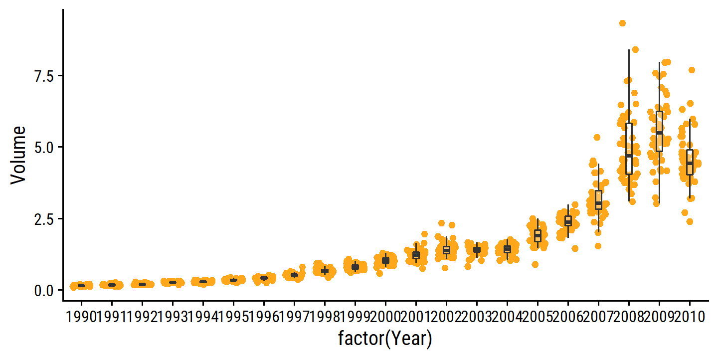

2. Logistic regression.

Before fitting, I will reverse the order of the Direction factor so that the first level is “Up” because tidymodels treats the first level as “positive.”

weekly <- weekly %>% mutate(Direction = fct_rev(Direction))

lr_weekly_fit <-
  logistic_reg() %>%
  fit(Direction ~ Year + Lag1 + Lag2 + Lag3 + Lag4 + Lag5 + Volume,
      data = weekly)
tidy_custom(lr_weekly_fit) %>%
  gt()

term	coefficient	std.error	z-statistic	p-value
(Intercept)	-17.2258	37.8905	-0.45	0.649
Year	0.0085	0.0190	0.45	0.654
Lag1	0.0407	0.0264	1.54	0.124
Lag2	-0.0594	0.0270	-2.20	0.028
Lag3	0.0155	0.0267	0.58	0.562
Lag4	0.0273	0.0265	1.03	0.302
Lag5	0.0140	0.0264	0.53	0.595
Volume	-0.0033	0.0688	-0.05	0.962

Only Lag2 was a significant predictor.

3. Confusion matrix.

lr_weekly_fit_conf_mat <- augment(lr_weekly_fit, weekly) %>%
  conf_mat(truth = Direction, estimate = .pred_class)
lr_weekly_fit_conf_mat

##           Truth
## Prediction  Up Down
##       Up   558  428
##       Down  47   56

• The model predicts many more Direction = “Up” than “Down”.
• The overall accuracy was slightly better than guessing: 56%.
• The sensitivity, TP / (TP + FP) was very good: 92%.
• The specificity, TN / (TN + FN) was very poor: 12%.

4. Logistic regression with Lag2 as the sole predictor.

Split into training and testing:

weekly_train <- weekly %>% filter(Year <= 2008)
weekly_test <- weekly %>% filter(Year > 2008)

lr_weekly_fit_lag2 <-
  logistic_reg() %>%
  fit(Direction ~ Lag2, data = weekly_train)
lr_weekly_fit_lag2_conf_mat <-
  augment(lr_weekly_fit_lag2, weekly_test) %>%
  conf_mat(truth = Direction, estimate = .pred_class)
lr_weekly_fit_lag2_conf_mat

##           Truth
## Prediction Up Down
##       Up   56   34
##       Down  5    9

• The model still predicts many more Direction = “Up” than “Down”.
• The overall accuracy: 62%.
• The sensitivity: 92%.
• The specificity: 21%.

(e-h) Repeat using LDA, QDA, KNN, naive Bayes.

model_fits <-
  list(
    "logistic" = lr_weekly_fit_lag2,
    "LDA" = discrim_linear() %>% fit(Direction ~ Lag2, data = weekly_train),
    "QDA" = discrim_quad() %>% fit(Direction ~ Lag2, data = weekly_train),
    "KNN1" = nearest_neighbor(mode = "classification", neighbors = 1) %>%
      fit(Direction ~ Lag2, data = weekly_train),
    "NB" = naive_Bayes() %>% fit(Direction ~ Lag2, data = weekly_train)
  )

weekly_metrics <- metric_set(accuracy, sens, spec, ppv)
imap_dfr(
  model_fits,
  ~augment(.x, new_data = weekly_test) %>%
    weekly_metrics(truth = Direction, estimate = .pred_class),
  .id = "model"
) %>%
  select(model, .metric, .estimate) %>%
  pivot_wider(names_from = .metric, values_from = .estimate) %>%
  gt(rowname_col = "model") %>%
  fmt_percent(columns = -model)

	accuracy	sens	spec	ppv
logistic	62.50%	91.80%	20.93%	62.22%
LDA	62.50%	91.80%	20.93%	62.22%
QDA	58.65%	100.00%	0.00%	58.65%
KNN1	50.00%	49.18%	51.16%	58.82%
NB	60.58%	91.80%	16.28%	60.87%

1. Which method was best?

• LDA and logistic regression performed exactly the same, and did the best.
• QDA predicted everything as “Up”.
• KNN with 1 neighbor was a coin flip simulator.
• Naive Bayes did slightly worse than logistic and LDA.

14. Predict gas mileage with Auto

1. Create a binary outcome mpg01.

auto <- ISLR2::Auto %>%
  mutate(mpg01 = ifelse(mpg > median(mpg), 1, 0),
         mpg01 = factor(mpg01))
glimpse(auto)

## Rows: 392
## Columns: 10
## $ mpg          <dbl> 18, 15, 18, 16, 17, 15, 14, 14, 14, 15, 15, 14, 15, 14, 2…
## $ cylinders    <int> 8, 8, 8, 8, 8, 8, 8, 8, 8, 8, 8, 8, 8, 8, 4, 6, 6, 6, 4, …
## $ displacement <dbl> 307, 350, 318, 304, 302, 429, 454, 440, 455, 390, 383, 34…
## $ horsepower   <int> 130, 165, 150, 150, 140, 198, 220, 215, 225, 190, 170, 16…
## $ weight       <int> 3504, 3693, 3436, 3433, 3449, 4341, 4354, 4312, 4425, 385…
## $ acceleration <dbl> 12.0, 11.5, 11.0, 12.0, 10.5, 10.0, 9.0, 8.5, 10.0, 8.5, …
## $ year         <int> 70, 70, 70, 70, 70, 70, 70, 70, 70, 70, 70, 70, 70, 70, 7…
## $ origin       <int> 1, 1, 1, 1, 1, 1, 1, 1, 1, 1, 1, 1, 1, 1, 3, 1, 1, 1, 3, …
## $ name         <fct> chevrolet chevelle malibu, buick skylark 320, plymouth sa…
## $ mpg01        <fct> 0, 0, 0, 0, 0, 0, 0, 0, 0, 0, 0, 0, 0, 0, 1, 0, 0, 0, 1, …

Note that origin is a numeric coding for 1. American, 2. European, and 3. Japanese, and so should be a factor:

auto <- auto %>%
  mutate(origin = factor(origin, levels = 1:3,
                         labels = c("American", "European", "Japanese")))

2. Explore the data.

auto %>%
  select(-name, -origin, -mpg) %>%
  pivot_longer(-mpg01, names_to = "var", values_to = "val") %>%
  ggplot(aes(y = mpg01, x = val)) +
  geom_boxplot(aes(fill = factor(mpg01))) +
  facet_wrap(~var, scales = "free_x") +
  theme(legend.position = "none") +
  add_facet_borders()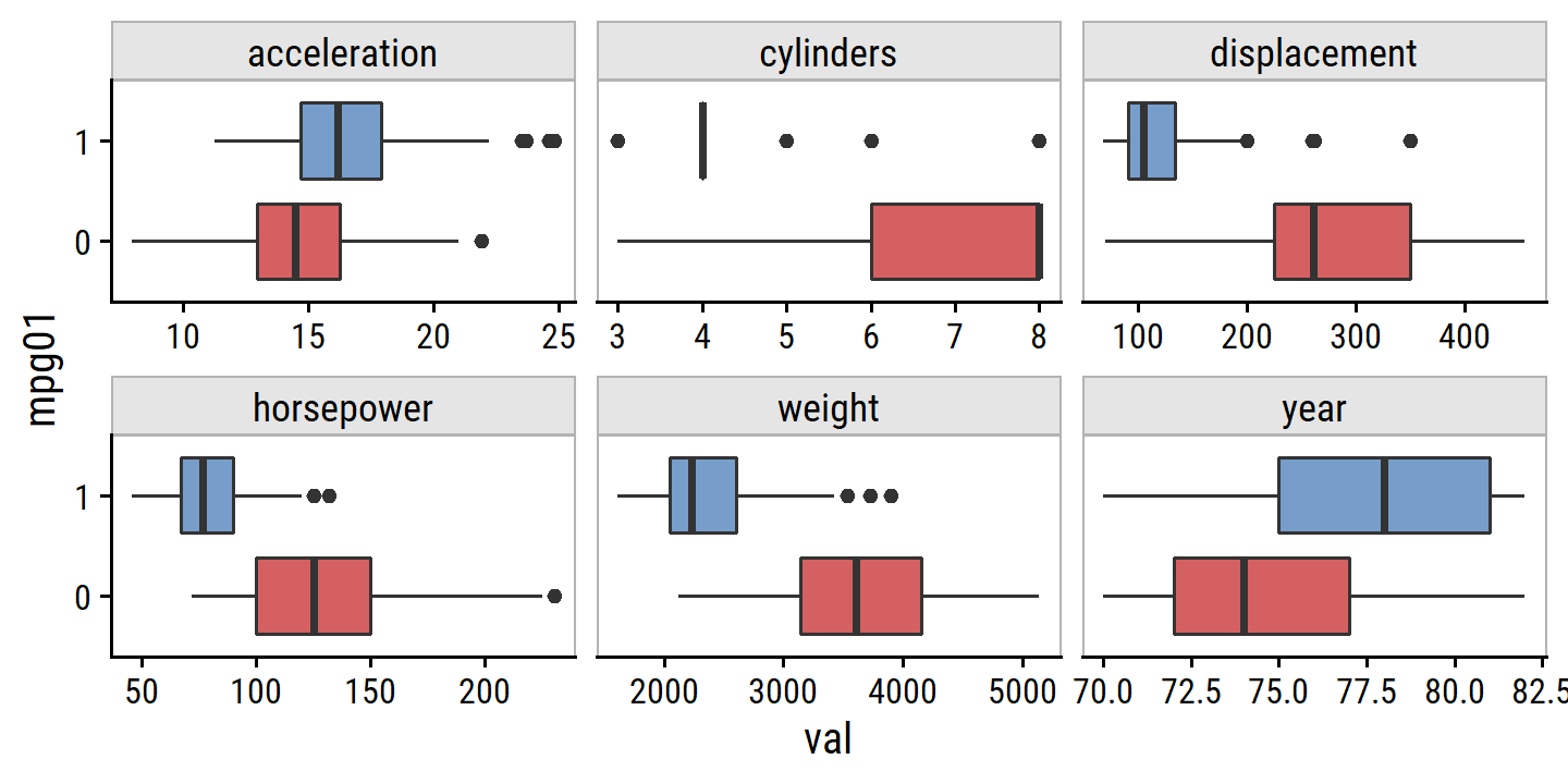

auto %>%
  count(origin, mpg01) %>%
  ggplot(aes(y = origin, x = mpg01)) +
  geom_tile(aes(fill = n)) +
  geom_text(aes(label = n), color = "white") +
  scale_x_discrete(expand = c(0, 0)) +
  scale_y_discrete(expand = c(0, 0)) +
  theme(legend.position = "none")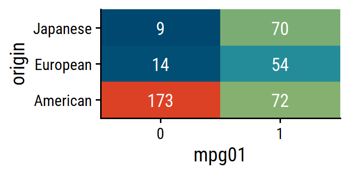

All of the variables here look useful for predicting mpg01, but cylinders, displacement, origin, and weight in particular.

Look at the correlation between variables:

auto %>% select(-name, -mpg01, -origin) %>%
  corrr::correlate(method = "pearson", quiet = TRUE) %>%
  gt(rowname_col = "term") %>%
  gt::fmt_missing(columns = everything(), missing_text = "") %>%
  gt::data_color(
    columns = everything(),
    colors = scales::col_numeric(
      palette = td_pal("div5")(5),
      domain = c(-1, 1)
    )
  ) %>%
  gt::fmt_number(columns = everything(), decimals = 2)

## Warning: The `fmt_missing()` function is deprecated and will soon be removed
## * Use the `sub_missing()` function instead

	mpg	cylinders	displacement	horsepower	weight	acceleration	year
mpg		−0.78	−0.81	−0.78	−0.83	0.42	0.58
cylinders	−0.78		0.95	0.84	0.90	−0.50	−0.35
displacement	−0.81	0.95		0.90	0.93	−0.54	−0.37
horsepower	−0.78	0.84	0.90		0.86	−0.69	−0.42
weight	−0.83	0.90	0.93	0.86		−0.42	−0.31
acceleration	0.42	−0.50	−0.54	−0.69	−0.42		0.29
year	0.58	−0.35	−0.37	−0.42	−0.31	0.29

Lots of inter-correlation.

3. Split the data into a training set and test set.

Use a 3:1 split:

set.seed(49)
auto_split <- initial_split(auto, prop = 3 / 4)
auto_train <- training(auto_split)
auto_test <- testing(auto_split)

Normally, I would set the strata argument to the output variable mpg01, but by construction (separated by the median) the data is split in half.

auto_train %>% count(mpg01)

##   mpg01   n
## 1     0 148
## 2     1 146

auto_test %>% count(mpg01)

##   mpg01  n
## 1     0 48
## 2     1 50

(d-h) Perform LDA, QDA, logistic regression, naive Bayes, and KNN.

Define the recipe, and add it to a generic workflow:

auto_recipe <- recipe(
  mpg01 ~ cylinders + displacement + horsepower + weight + acceleration +
    year + origin,
  data = auto_train
) %>%
  # Normalize numerical predictors to work with KNN
  step_normalize(all_numeric_predictors()) %>%
  step_dummy(origin)
auto_workflow <- workflow() %>%
  add_recipe(auto_recipe)

Fit and summarize metrics:

model_fits <-
  list(
    "LDA" = auto_workflow %>%
      add_model(discrim_linear()) %>%
      fit(data = auto_train),
    "QDA" = auto_workflow %>%
      add_model(discrim_quad()) %>%
      fit(data = auto_train),
    "logistic" = auto_workflow %>%
      add_model(logistic_reg()) %>%
      fit(data = auto_train),
    "NB" = auto_workflow %>%
      add_model(naive_Bayes()) %>%
      fit(data = auto_train),
    "KNN1" = auto_workflow %>%
      add_model(nearest_neighbor(mode = "classification", neighbors = 1)) %>%
      fit(data = auto_train),
    "KNN3" = auto_workflow %>%
      add_model(nearest_neighbor(mode = "classification", neighbors = 3)) %>%
      fit(data = auto_train),
    "KNN5" = auto_workflow %>%
      add_model(nearest_neighbor(mode = "classification", neighbors = 5)) %>%
      fit(data = auto_train),
    "KNN7" = auto_workflow %>%
      add_model(nearest_neighbor(mode = "classification", neighbors = 7)) %>%
      fit(data = auto_train)
  )
auto_metrics <- metric_set(accuracy, sens, spec, ppv)
imap_dfr(
  model_fits,
  ~augment(.x, new_data = auto_test) %>%
    auto_metrics(truth = mpg01, estimate = .pred_class),
  .id = "model"
) %>%
  select(model, .metric, .estimate) %>%
  pivot_wider(names_from = .metric, values_from = .estimate) %>%
  arrange(desc(accuracy)) %>%
  gt(rowname_col = "model") %>%
  fmt_percent(columns = -model, decimals = 1)

	accuracy	sens	spec	ppv
LDA	90.8%	87.5%	94.0%	93.3%
logistic	90.8%	91.7%	90.0%	89.8%
QDA	89.8%	85.4%	94.0%	93.2%
NB	89.8%	87.5%	92.0%	91.3%
KNN1	89.8%	93.8%	86.0%	86.5%
KNN3	89.8%	93.8%	86.0%	86.5%
KNN5	89.8%	91.7%	88.0%	88.0%
KNN7	89.8%	91.7%	88.0%	88.0%

All models did well, but LDA and logistic regression were the best. There wasn’t any difference in KNN accuracy for \(K\) = 1, 3, 5, and 7.

16. Predict crime rate with Boston

boston <- ISLR2::Boston %>%
  mutate(
    crim01 = ifelse(crim > median(crim), 1, 0),
    crim01 = factor(crim01),
    # Convert the binary chas variable to TRUE/FALSE
    chas = chas == 1
  )
glimpse(boston)

## Rows: 506
## Columns: 14
## $ crim    <dbl> 0.00632, 0.02731, 0.02729, 0.03237, 0.06905, 0.02985, 0.08829,…
## $ zn      <dbl> 18.0, 0.0, 0.0, 0.0, 0.0, 0.0, 12.5, 12.5, 12.5, 12.5, 12.5, 1…
## $ indus   <dbl> 2.31, 7.07, 7.07, 2.18, 2.18, 2.18, 7.87, 7.87, 7.87, 7.87, 7.…
## $ chas    <lgl> FALSE, FALSE, FALSE, FALSE, FALSE, FALSE, FALSE, FALSE, FALSE,…
## $ nox     <dbl> 0.538, 0.469, 0.469, 0.458, 0.458, 0.458, 0.524, 0.524, 0.524,…
## $ rm      <dbl> 6.575, 6.421, 7.185, 6.998, 7.147, 6.430, 6.012, 6.172, 5.631,…
## $ age     <dbl> 65.2, 78.9, 61.1, 45.8, 54.2, 58.7, 66.6, 96.1, 100.0, 85.9, 9…
## $ dis     <dbl> 4.0900, 4.9671, 4.9671, 6.0622, 6.0622, 6.0622, 5.5605, 5.9505…
## $ rad     <int> 1, 2, 2, 3, 3, 3, 5, 5, 5, 5, 5, 5, 5, 4, 4, 4, 4, 4, 4, 4, 4,…
## $ tax     <dbl> 296, 242, 242, 222, 222, 222, 311, 311, 311, 311, 311, 311, 31…
## $ ptratio <dbl> 15.3, 17.8, 17.8, 18.7, 18.7, 18.7, 15.2, 15.2, 15.2, 15.2, 15…
## $ lstat   <dbl> 4.98, 9.14, 4.03, 2.94, 5.33, 5.21, 12.43, 19.15, 29.93, 17.10…
## $ medv    <dbl> 24.0, 21.6, 34.7, 33.4, 36.2, 28.7, 22.9, 27.1, 16.5, 18.9, 15…
## $ crim01  <fct> 0, 0, 0, 0, 0, 0, 0, 0, 0, 0, 0, 0, 0, 1, 1, 1, 1, 1, 1, 1, 1,…

boston %>%
  select(-chas) %>%
  pivot_longer(-crim01, names_to = "var", values_to = "val") %>%
  ggplot(aes(y = crim01, x = val)) +
  geom_boxplot(aes(fill = factor(crim01))) +
  facet_wrap(~var, scales = "free_x") +
  theme(legend.position = "none") +
  add_facet_borders()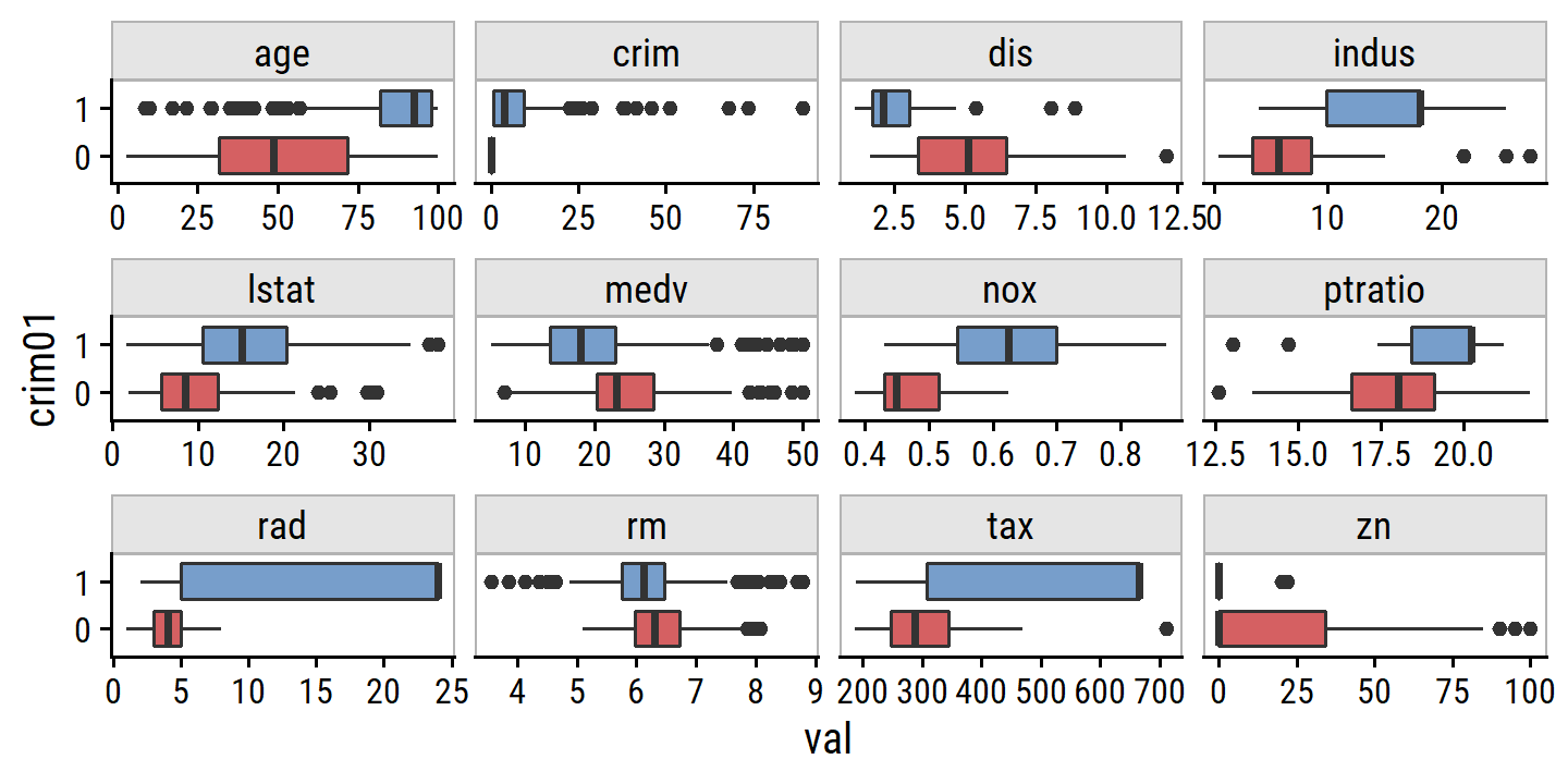

boston %>%
  count(chas, crim01) %>%
  ggplot(aes(y = chas, x = crim01)) +
  geom_tile(aes(fill = n)) +
  geom_text(aes(label = n), color = "white") +
  scale_x_discrete(expand = c(0, 0)) +
  scale_y_discrete(expand = c(0, 0)) +
  theme(legend.position = "none")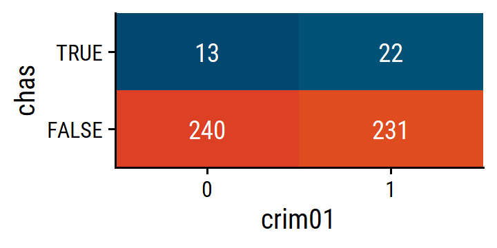

The chas and rm (average number of rooms per dwelling) variables look the least useful of these predictors. Split the data:

set.seed(98)
# By default, splits 3:1
boston_split <- initial_split(boston)
boston_train <- training(boston_split)
boston_test <- testing(boston_split)

Fit and summarize metrics for all the models and a few different predictor sets:

boston_models <- list(
  "LDA" = discrim_linear(),
  "QDA" = discrim_quad(),
  "logistic" = logistic_reg(),
  "NB" = naive_Bayes(),
  "KNN1" = nearest_neighbor(mode = "classification", neighbors = 1),
  "KNN3" = nearest_neighbor(mode = "classification", neighbors = 3),
  "KNN5" = nearest_neighbor(mode = "classification", neighbors = 5),
  "KNN7" = nearest_neighbor(mode = "classification", neighbors = 7)
)
boston_recs <- list(
  "rec1" = recipe(
    crim01 ~ age + dis + indus + lstat + medv + nox + ptratio + rad + tax + zn,
    data = boston_train
  ) %>%
    step_normalize(all_numeric_predictors()),
  # Drop medv and lstat
  "rec2" = recipe(
    crim01 ~ age + dis + indus + nox + ptratio + rad + tax + zn,
    data = boston_train
  ) %>%
    step_normalize(all_numeric_predictors()),
  # Drop ptratio and tax
  "rec3" = recipe(
    crim01 ~ age + dis + indus + nox  + rad + zn,
    data = boston_train
  ) %>%
    step_normalize(all_numeric_predictors())
)

boston_fits <-
  map(
    boston_models,
    function(model) {
      map(
        boston_recs,
        ~workflow() %>%
          add_model(model) %>%
          add_recipe(.x) %>%
          fit(data = boston_train)
      )
    }
  )

boston_metrics <- metric_set(accuracy, sens, spec, ppv)
imap_dfr(
  boston_fits,
  function(fit, y) {
    imap_dfr(
      fit,
      ~augment(.x, new_data = boston_test) %>%
        boston_metrics(truth = crim01, estimate = .pred_class),
      .id = "recipe"
    )
  },
  .id = "model"
) %>%
  select(model, recipe, .metric, .estimate) %>%
  pivot_wider(names_from = .metric, values_from = .estimate) %>%
  arrange(recipe, desc(accuracy)) %>%
  group_by(recipe) %>%
  gt(rowname_col = "model") %>%
  fmt_percent(columns = -model, decimals = 1)

	accuracy	sens	spec	ppv
rec1
QDA	95.3%	94.6%	95.8%	94.6%
KNN1	94.5%	98.2%	91.5%	90.2%
KNN3	94.5%	98.2%	91.5%	90.2%
KNN5	94.5%	98.2%	91.5%	90.2%
KNN7	94.5%	98.2%	91.5%	90.2%
logistic	92.1%	98.2%	87.3%	85.9%
NB	85.0%	80.4%	88.7%	84.9%
LDA	83.5%	91.1%	77.5%	76.1%
rec2
KNN5	96.1%	100.0%	93.0%	91.8%
KNN1	95.3%	98.2%	93.0%	91.7%
KNN3	95.3%	98.2%	93.0%	91.7%
KNN7	95.3%	98.2%	93.0%	91.7%
QDA	94.5%	94.6%	94.4%	93.0%
logistic	89.0%	87.5%	90.1%	87.5%
LDA	86.6%	96.4%	78.9%	78.3%
NB	84.3%	80.4%	87.3%	83.3%
rec3
KNN5	95.3%	98.2%	93.0%	91.7%
KNN1	94.5%	98.2%	91.5%	90.2%
KNN3	94.5%	98.2%	91.5%	90.2%
KNN7	94.5%	96.4%	93.0%	91.5%
logistic	89.0%	87.5%	90.1%	87.5%
QDA	86.6%	91.1%	83.1%	81.0%
NB	86.6%	76.8%	94.4%	91.5%
LDA	84.3%	91.1%	78.9%	77.3%

In general, performance was best for rec2 with these variables:

boston_recs$rec2$term_info

## # A tibble: 9 × 4
##   variable type    role      source  
##   <chr>    <chr>   <chr>     <chr>   
## 1 age      numeric predictor original
## 2 dis      numeric predictor original
## 3 indus    numeric predictor original
## 4 nox      numeric predictor original
## 5 ptratio  numeric predictor original
## 6 rad      numeric predictor original
## 7 tax      numeric predictor original
## 8 zn       numeric predictor original
## 9 crim01   nominal outcome   original

And the models that performed best were KNN and QDA.

Reproducibility

Reproducibility receipt

Sys.time()

## [1] "2022-09-19 10:28:39 AST"

if ("git2r" %in% installed.packages()) {
  if (git2r::in_repository()) {
    git2r::repository()
  }
}

## Local:    main C:/Users/tdunn/Documents/learning/islr-tidy
## Remote:   main @ origin (https://github.com/taylordunn/islr-tidy)
## Head:     [b60974c] 2022-09-19: Working on the empirical examples in Chapter 4 (issue #1)

sessioninfo::session_info()

## ─ Session info ───────────────────────────────────────────────────────────────
##  setting  value
##  version  R version 4.2.1 (2022-06-23 ucrt)
##  os       Windows 10 x64 (build 19044)
##  system   x86_64, mingw32
##  ui       RTerm
##  language (EN)
##  collate  English_Canada.utf8
##  ctype    English_Canada.utf8
##  tz       America/Curacao
##  date     2022-09-19
##  pandoc   2.18 @ C:/Program Files/RStudio/bin/quarto/bin/tools/ (via rmarkdown)
## 
## ─ Packages ───────────────────────────────────────────────────────────────────
##  package        * version    date (UTC) lib source
##  abind            1.4-5      2016-07-21 [1] CRAN (R 4.2.0)
##  assertthat       0.2.1      2019-03-21 [1] CRAN (R 4.2.1)
##  backports        1.4.1      2021-12-13 [1] CRAN (R 4.2.0)
##  base64enc        0.1-3      2015-07-28 [1] CRAN (R 4.2.0)
##  bayestestR       0.12.1     2022-05-02 [1] CRAN (R 4.2.1)
##  bit              4.0.4      2020-08-04 [1] CRAN (R 4.2.1)
##  bit64            4.0.5      2020-08-30 [1] CRAN (R 4.2.1)
##  bookdown         0.27       2022-06-14 [1] CRAN (R 4.2.1)
##  broom          * 1.0.0      2022-07-01 [1] CRAN (R 4.2.1)
##  bslib            0.4.0      2022-07-16 [1] CRAN (R 4.2.1)
##  cachem           1.0.6      2021-08-19 [1] CRAN (R 4.2.1)
##  car              3.1-0      2022-06-15 [1] CRAN (R 4.2.1)
##  carData          3.0-5      2022-01-06 [1] CRAN (R 4.2.1)
##  cellranger       1.1.0      2016-07-27 [1] CRAN (R 4.2.1)
##  checkmate        2.1.0      2022-04-21 [1] CRAN (R 4.2.1)
##  class            7.3-20     2022-01-16 [2] CRAN (R 4.2.1)
##  cli              3.3.0      2022-04-25 [1] CRAN (R 4.2.1)
##  codetools        0.2-18     2020-11-04 [2] CRAN (R 4.2.1)
##  colorspace       2.0-3      2022-02-21 [1] CRAN (R 4.2.1)
##  combinat         0.0-8      2012-10-29 [1] CRAN (R 4.2.0)
##  corrr          * 0.4.4      2022-08-16 [1] CRAN (R 4.2.1)
##  crayon           1.5.1      2022-03-26 [1] CRAN (R 4.2.1)
##  datawizard       0.4.1      2022-05-16 [1] CRAN (R 4.2.1)
##  DBI              1.1.3      2022-06-18 [1] CRAN (R 4.2.1)
##  dbplyr           2.2.1      2022-06-27 [1] CRAN (R 4.2.1)
##  dials          * 1.0.0      2022-06-14 [1] CRAN (R 4.2.1)
##  DiceDesign       1.9        2021-02-13 [1] CRAN (R 4.2.1)
##  digest           0.6.29     2021-12-01 [1] CRAN (R 4.2.1)
##  discrim        * 1.0.0      2022-06-23 [1] CRAN (R 4.2.1)
##  distill          1.4        2022-05-12 [1] CRAN (R 4.2.1)
##  distributional   0.3.0      2022-01-05 [1] CRAN (R 4.2.1)
##  downlit          0.4.2      2022-07-05 [1] CRAN (R 4.2.1)
##  dplyr          * 1.0.9      2022-04-28 [1] CRAN (R 4.2.1)
##  dunnr          * 0.2.6      2022-08-07 [1] Github (taylordunn/dunnr@e2a8213)
##  ellipsis         0.3.2      2021-04-29 [1] CRAN (R 4.2.1)
##  equatiomatic     0.3.1      2022-01-30 [1] CRAN (R 4.2.1)
##  evaluate         0.15       2022-02-18 [1] CRAN (R 4.2.1)
##  extrafont        0.18       2022-04-12 [1] CRAN (R 4.2.0)
##  extrafontdb      1.0        2012-06-11 [1] CRAN (R 4.2.0)
##  fansi            1.0.3      2022-03-24 [1] CRAN (R 4.2.1)
##  farver           2.1.1      2022-07-06 [1] CRAN (R 4.2.1)
##  fastmap          1.1.0      2021-01-25 [1] CRAN (R 4.2.1)
##  forcats        * 0.5.1      2021-01-27 [1] CRAN (R 4.2.1)
##  foreach          1.5.2      2022-02-02 [1] CRAN (R 4.2.1)
##  fs               1.5.2      2021-12-08 [1] CRAN (R 4.2.1)
##  furrr            0.3.0      2022-05-04 [1] CRAN (R 4.2.1)
##  future           1.27.0     2022-07-22 [1] CRAN (R 4.2.1)
##  future.apply     1.9.0      2022-04-25 [1] CRAN (R 4.2.1)
##  gargle           1.2.0      2021-07-02 [1] CRAN (R 4.2.1)
##  generics         0.1.3      2022-07-05 [1] CRAN (R 4.2.1)
##  GGally           2.1.2      2021-06-21 [1] CRAN (R 4.2.1)
##  ggdist         * 3.2.0      2022-07-19 [1] CRAN (R 4.2.1)
##  ggplot2        * 3.3.6      2022-05-03 [1] CRAN (R 4.2.1)
##  ggrepel          0.9.1      2021-01-15 [1] CRAN (R 4.2.1)
##  git2r            0.30.1     2022-03-16 [1] CRAN (R 4.2.1)
##  globals          0.15.1     2022-06-24 [1] CRAN (R 4.2.1)
##  glue             1.6.2      2022-02-24 [1] CRAN (R 4.2.1)
##  googledrive      2.0.0      2021-07-08 [1] CRAN (R 4.2.1)
##  googlesheets4    1.0.0      2021-07-21 [1] CRAN (R 4.2.1)
##  gower            1.0.0      2022-02-03 [1] CRAN (R 4.2.0)
##  GPfit            1.0-8      2019-02-08 [1] CRAN (R 4.2.1)
##  gt             * 0.6.0      2022-05-24 [1] CRAN (R 4.2.1)
##  gtable           0.3.0      2019-03-25 [1] CRAN (R 4.2.1)
##  hardhat          1.2.0      2022-06-30 [1] CRAN (R 4.2.1)
##  haven            2.5.0      2022-04-15 [1] CRAN (R 4.2.1)
##  here           * 1.0.1      2020-12-13 [1] CRAN (R 4.2.1)
##  highr            0.9        2021-04-16 [1] CRAN (R 4.2.1)
##  hms              1.1.1      2021-09-26 [1] CRAN (R 4.2.1)
##  htmltools        0.5.2      2021-08-25 [1] CRAN (R 4.2.1)
##  httpuv           1.6.5      2022-01-05 [1] CRAN (R 4.2.1)
##  httr             1.4.3      2022-05-04 [1] CRAN (R 4.2.1)
##  igraph           1.3.4      2022-07-19 [1] CRAN (R 4.2.1)
##  infer          * 1.0.2      2022-06-10 [1] CRAN (R 4.2.1)
##  insight          0.18.0     2022-07-05 [1] CRAN (R 4.2.1)
##  ipred            0.9-13     2022-06-02 [1] CRAN (R 4.2.1)
##  ISLR2          * 1.3-1      2022-01-10 [1] CRAN (R 4.2.1)
##  iterators        1.0.14     2022-02-05 [1] CRAN (R 4.2.1)
##  jquerylib        0.1.4      2021-04-26 [1] CRAN (R 4.2.1)
##  jsonlite         1.8.0      2022-02-22 [1] CRAN (R 4.2.1)
##  kknn             1.3.1      2016-03-26 [1] CRAN (R 4.2.1)
##  klaR             1.7-1      2022-06-27 [1] CRAN (R 4.2.1)
##  knitr            1.39       2022-04-26 [1] CRAN (R 4.2.1)
##  labeling         0.4.2      2020-10-20 [1] CRAN (R 4.2.0)
##  labelled         2.9.1      2022-05-05 [1] CRAN (R 4.2.1)
##  later            1.3.0      2021-08-18 [1] CRAN (R 4.2.1)
##  lattice          0.20-45    2021-09-22 [2] CRAN (R 4.2.1)
##  lava             1.6.10     2021-09-02 [1] CRAN (R 4.2.1)
##  lhs              1.1.5      2022-03-22 [1] CRAN (R 4.2.1)
##  lifecycle        1.0.1      2021-09-24 [1] CRAN (R 4.2.1)
##  listenv          0.8.0      2019-12-05 [1] CRAN (R 4.2.1)
##  lubridate        1.8.0      2021-10-07 [1] CRAN (R 4.2.1)
##  magrittr         2.0.3      2022-03-30 [1] CRAN (R 4.2.1)
##  MASS             7.3-57     2022-04-22 [2] CRAN (R 4.2.1)
##  Matrix           1.4-1      2022-03-23 [2] CRAN (R 4.2.1)
##  memoise          2.0.1      2021-11-26 [1] CRAN (R 4.2.1)
##  mgcv             1.8-40     2022-03-29 [2] CRAN (R 4.2.1)
##  mime             0.12       2021-09-28 [1] CRAN (R 4.2.0)
##  miniUI           0.1.1.1    2018-05-18 [1] CRAN (R 4.2.1)
##  modeldata      * 1.0.0      2022-07-01 [1] CRAN (R 4.2.1)
##  modelr           0.1.8      2020-05-19 [1] CRAN (R 4.2.1)
##  munsell          0.5.0      2018-06-12 [1] CRAN (R 4.2.1)
##  mvtnorm          1.1-3      2021-10-08 [1] CRAN (R 4.2.0)
##  nlme             3.1-157    2022-03-25 [2] CRAN (R 4.2.1)
##  nnet             7.3-17     2022-01-16 [2] CRAN (R 4.2.1)
##  parallelly       1.32.1     2022-07-21 [1] CRAN (R 4.2.1)
##  parsnip        * 1.0.0      2022-06-16 [1] CRAN (R 4.2.1)
##  patchwork      * 1.1.1      2020-12-17 [1] CRAN (R 4.2.1)
##  performance      0.9.1      2022-06-20 [1] CRAN (R 4.2.1)
##  pillar           1.8.0      2022-07-18 [1] CRAN (R 4.2.1)
##  pkgconfig        2.0.3      2019-09-22 [1] CRAN (R 4.2.1)
##  plyr             1.8.7      2022-03-24 [1] CRAN (R 4.2.1)
##  poissonreg     * 1.0.0      2022-06-15 [1] CRAN (R 4.2.1)
##  prodlim          2019.11.13 2019-11-17 [1] CRAN (R 4.2.1)
##  promises         1.2.0.1    2021-02-11 [1] CRAN (R 4.2.1)
##  purrr          * 0.3.4      2020-04-17 [1] CRAN (R 4.2.1)
##  questionr        0.7.7      2022-01-31 [1] CRAN (R 4.2.1)
##  R6               2.5.1      2021-08-19 [1] CRAN (R 4.2.1)
##  RColorBrewer     1.1-3      2022-04-03 [1] CRAN (R 4.2.0)
##  Rcpp             1.0.9      2022-07-08 [1] CRAN (R 4.2.1)
##  readr          * 2.1.2      2022-01-30 [1] CRAN (R 4.2.1)
##  readxl           1.4.0      2022-03-28 [1] CRAN (R 4.2.1)
##  recipes        * 1.0.1      2022-07-07 [1] CRAN (R 4.2.1)
##  repr             1.1.4      2022-01-04 [1] CRAN (R 4.2.1)
##  reprex           2.0.1      2021-08-05 [1] CRAN (R 4.2.1)
##  reshape          0.8.9      2022-04-12 [1] CRAN (R 4.2.1)
##  rlang            1.0.4      2022-07-12 [1] CRAN (R 4.2.1)
##  rmarkdown        2.14       2022-04-25 [1] CRAN (R 4.2.1)
##  rpart            4.1.16     2022-01-24 [2] CRAN (R 4.2.1)
##  rprojroot        2.0.3      2022-04-02 [1] CRAN (R 4.2.1)
##  rsample        * 1.1.0      2022-08-08 [1] CRAN (R 4.2.1)
##  rstudioapi       0.13       2020-11-12 [1] CRAN (R 4.2.1)
##  Rttf2pt1         1.3.8      2020-01-10 [1] CRAN (R 4.2.1)
##  rvest            1.0.2      2021-10-16 [1] CRAN (R 4.2.1)
##  sass             0.4.2      2022-07-16 [1] CRAN (R 4.2.1)
##  scales         * 1.2.0      2022-04-13 [1] CRAN (R 4.2.1)
##  see              0.7.1      2022-06-20 [1] CRAN (R 4.2.1)
##  sessioninfo      1.2.2      2021-12-06 [1] CRAN (R 4.2.1)
##  shiny            1.7.2      2022-07-19 [1] CRAN (R 4.2.1)
##  skimr            2.1.4      2022-04-15 [1] CRAN (R 4.2.1)
##  stringi          1.7.8      2022-07-11 [1] CRAN (R 4.2.1)
##  stringr        * 1.4.0      2019-02-10 [1] CRAN (R 4.2.1)
##  survival         3.3-1      2022-03-03 [2] CRAN (R 4.2.1)
##  tibble         * 3.1.8      2022-07-22 [1] CRAN (R 4.2.1)
##  tictoc         * 1.0.1      2021-04-19 [1] CRAN (R 4.2.0)
##  tidymodels     * 1.0.0      2022-07-13 [1] CRAN (R 4.2.1)
##  tidyr          * 1.2.0      2022-02-01 [1] CRAN (R 4.2.1)
##  tidyselect       1.1.2      2022-02-21 [1] CRAN (R 4.2.1)
##  tidyverse      * 1.3.2      2022-07-18 [1] CRAN (R 4.2.1)
##  timeDate         4021.104   2022-07-19 [1] CRAN (R 4.2.1)
##  tune           * 1.0.0      2022-07-07 [1] CRAN (R 4.2.1)
##  tzdb             0.3.0      2022-03-28 [1] CRAN (R 4.2.1)
##  usethis          2.1.6      2022-05-25 [1] CRAN (R 4.2.1)
##  utf8             1.2.2      2021-07-24 [1] CRAN (R 4.2.1)
##  vctrs            0.4.1      2022-04-13 [1] CRAN (R 4.2.1)
##  vroom            1.5.7      2021-11-30 [1] CRAN (R 4.2.1)
##  withr            2.5.0      2022-03-03 [1] CRAN (R 4.2.1)
##  workflows      * 1.0.0      2022-07-05 [1] CRAN (R 4.2.1)
##  workflowsets   * 1.0.0      2022-07-12 [1] CRAN (R 4.2.1)
##  xfun             0.31       2022-05-10 [1] CRAN (R 4.2.1)
##  xml2             1.3.3      2021-11-30 [1] CRAN (R 4.2.1)
##  xtable           1.8-4      2019-04-21 [1] CRAN (R 4.2.1)
##  yaml             2.3.5      2022-02-21 [1] CRAN (R 4.2.0)
##  yardstick      * 1.0.0      2022-06-06 [1] CRAN (R 4.2.1)
## 
##  [1] C:/Users/tdunn/AppData/Local/R/win-library/4.2
##  [2] C:/Program Files/R/R-4.2.1/library
## 
## ──────────────────────────────────────────────────────────────────────────────