Chapter 5 🔧 Continuous Random Variable

Figure 5.1: ‘Statistical Cow’ by Enrico Chavez

5.1 Two Motivating Examples

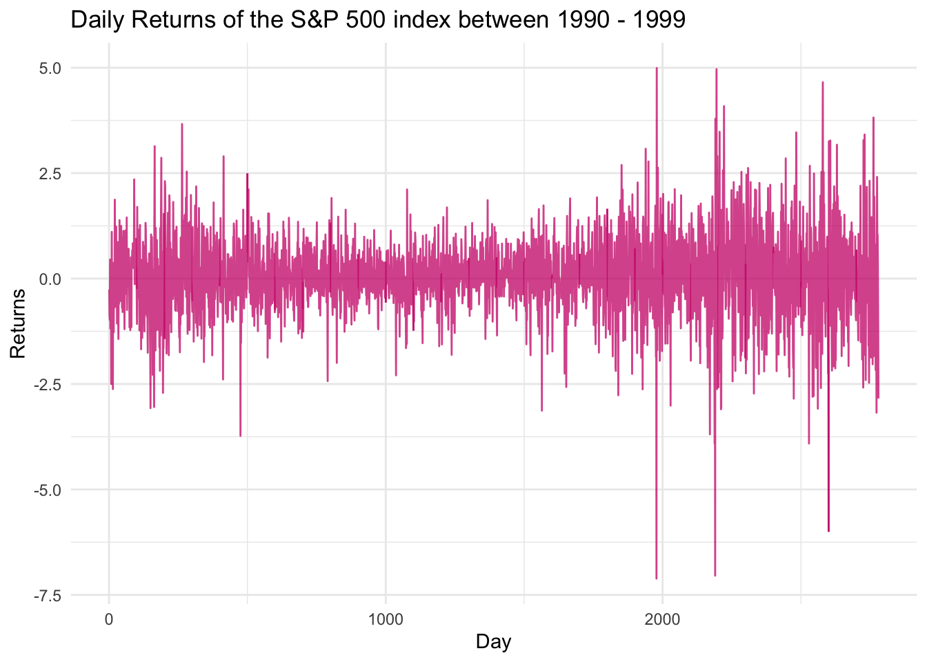
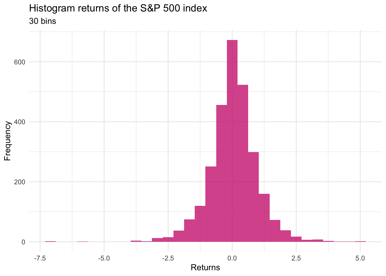
Let’s try to count the relative frequency of each of these returns, in an attempt to estimate the probability of each value of the return.

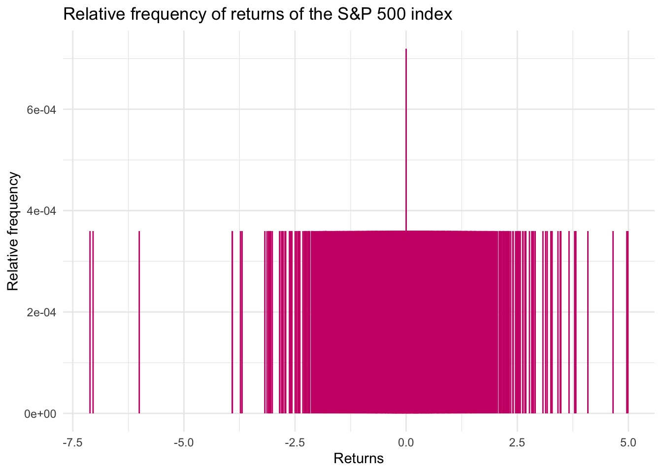
We notice that there are too many different values for the returns. This yields a low value and “uniform” relative frequency which does not help us gain any insight on the probability distribution of the values. Moreover, we could be almost sure that a future return would not have any of the values already obtained.

However, we notice that there’s some concentration, i.e. there are more returns in the neighborhood of zero, as there are in the extreme corners of the possible values. To quantify this concentration, we can create a histogram by splitting the space of possible values into a given number of intervals, or “bins”, and counting the number of observations within a bin.

If we consider 30 bins, we obtain the following plot:

If we consider separating the space of returns into 300 bins, we obtain the following plot:

We could go further and affine the number of bins and the method of counting. One of the options is to estimate a so-called Density Curve, which among other considerations, chooses to split the space into an infinite amount of bins.

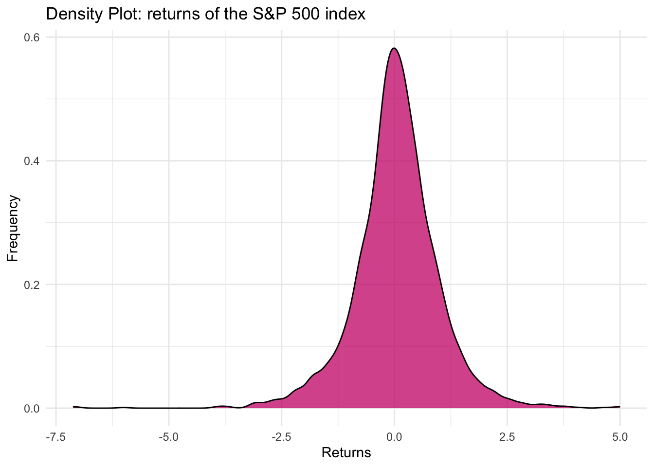
This plot is much more interesting, as it clearly shows that the returns are quite concentrated around 0.

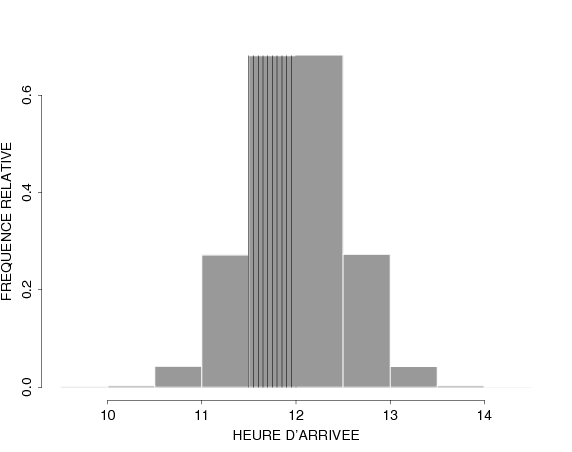
And we can affine our analysis by increasing the number of bins.

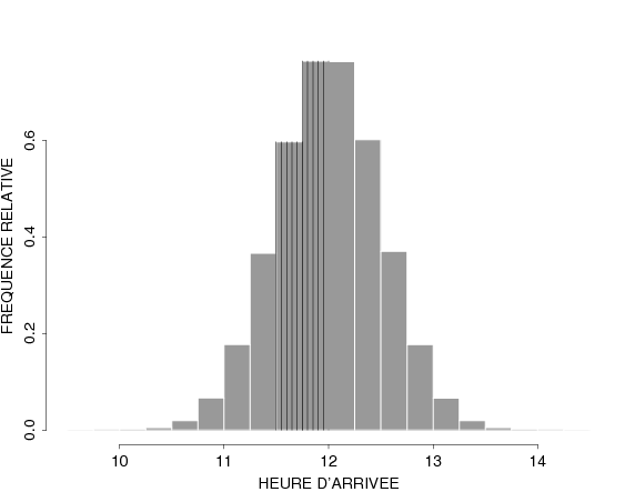
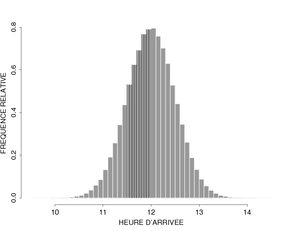
In the last one, we see that there is clearly a peak around 12h. If we would like to allocate resources (e.g. hire more service workers to adapt to the demand), we’d like to call the workers to provide service around those hours.

These examples are illustrations of a class of random variables which are different from what we have seen so far. Specifically, the examples emphasise that, unlike discrete random variables, the considered variables are continuous random variables i.e. they can take any value in an interval.

This means we cannot simply list all possible values of the random variable, because there are (infinitely many) an uncountable number of possible outcomes that might occur.

However, what we can do is to construct a probability distribution by assigning a positive probability to each and every possible interval of values that can occur. This is done by defining the Cumulative Distribution Function (CDF), which is sometimes called Probability Distribution Function.

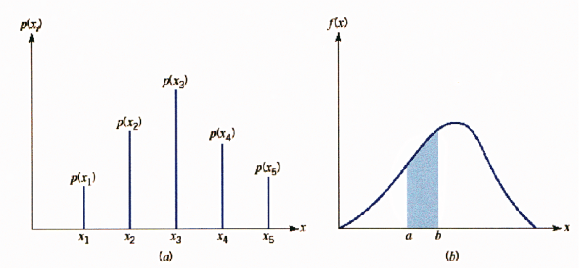
So, graphically, we have that the Discrete Random Variables have a distribution that allocates the probability to the values, represented by bars, whereas Continuous Random Variables have a distribution that allocates probability to intervals, represented by the area below the density curve enclosed by the interval.

5.2 Cumulative Distribution Function (CDF)

Graphically, if we represent the values of the PDF with a curve, the CDF will be the area beneath it in the interval considered.

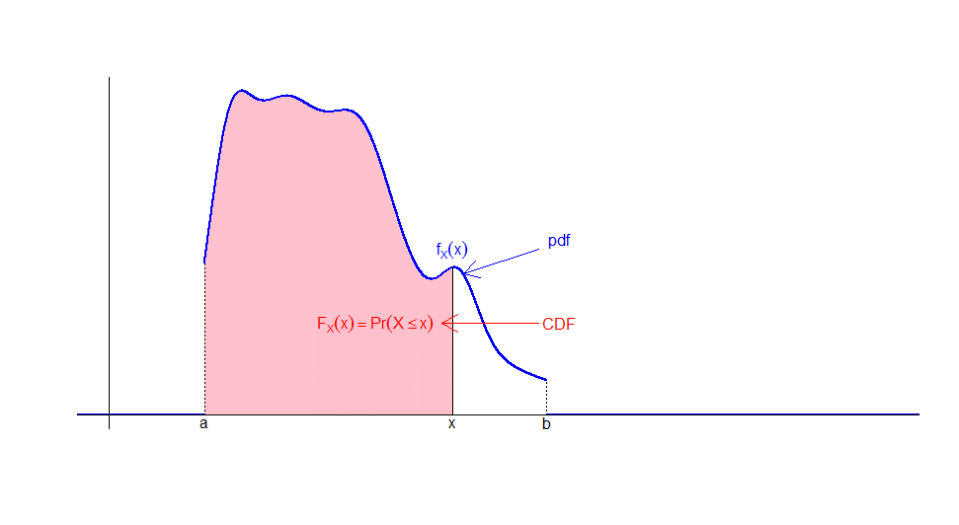
Another way of seeing this relationship is with the following plot, where the value of the area undereneath the density is mapped into a new curve that will represent the CDF.

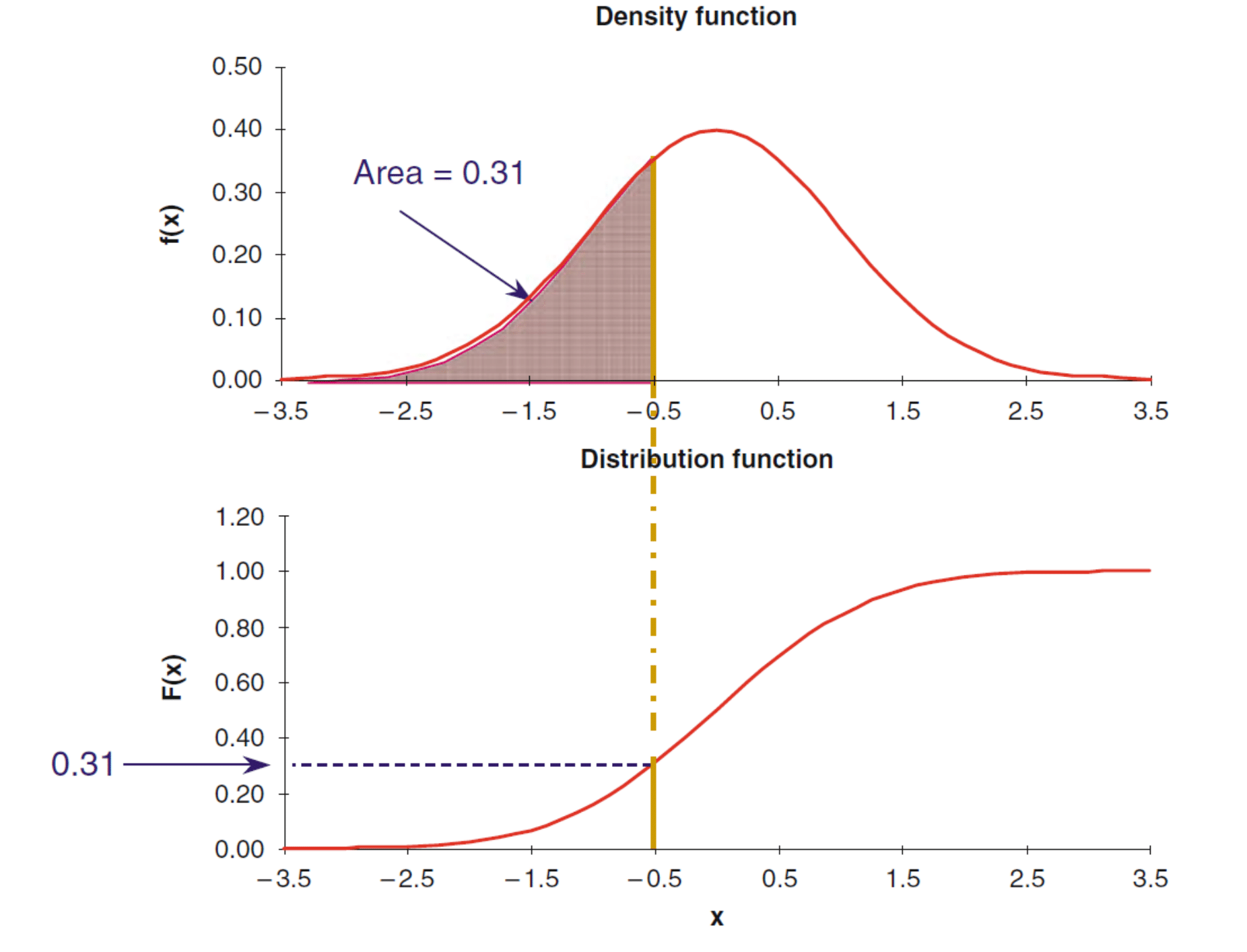
From a formal mathematical standpoint, the relationship between PDF and CDF is given by the fundamental theorem of integral calculus. In the illustration, \(X\) is a random variable taking values in the interval \((a,b]\), and the PDF \(f_{X}\left(x\right)\) is non-zero only in \((a,b)\). More generally we have, for a variable taking values on the whole real line (\(\mathbb{R}\)):

• the fundamental theorem of integral calculus yields \[\color{red}{F_{X}\left( x\right)} =P\left( X\leq x\right) =\int_{-\infty}^{x}\color{blue}{f_{X}\left( t\right)}dt,\] the area under the CDF between \(-\infty\) and \(x\)

• or in terms of derivative \[\color{blue}{f_{X}\left( x\right)} = \frac{d\color{red}{F_{X}(x)}}{dx}\]

Most of the PDF’s that we are going to consider are bell-shaped. So, typically, we will have a density that looks like a bell:

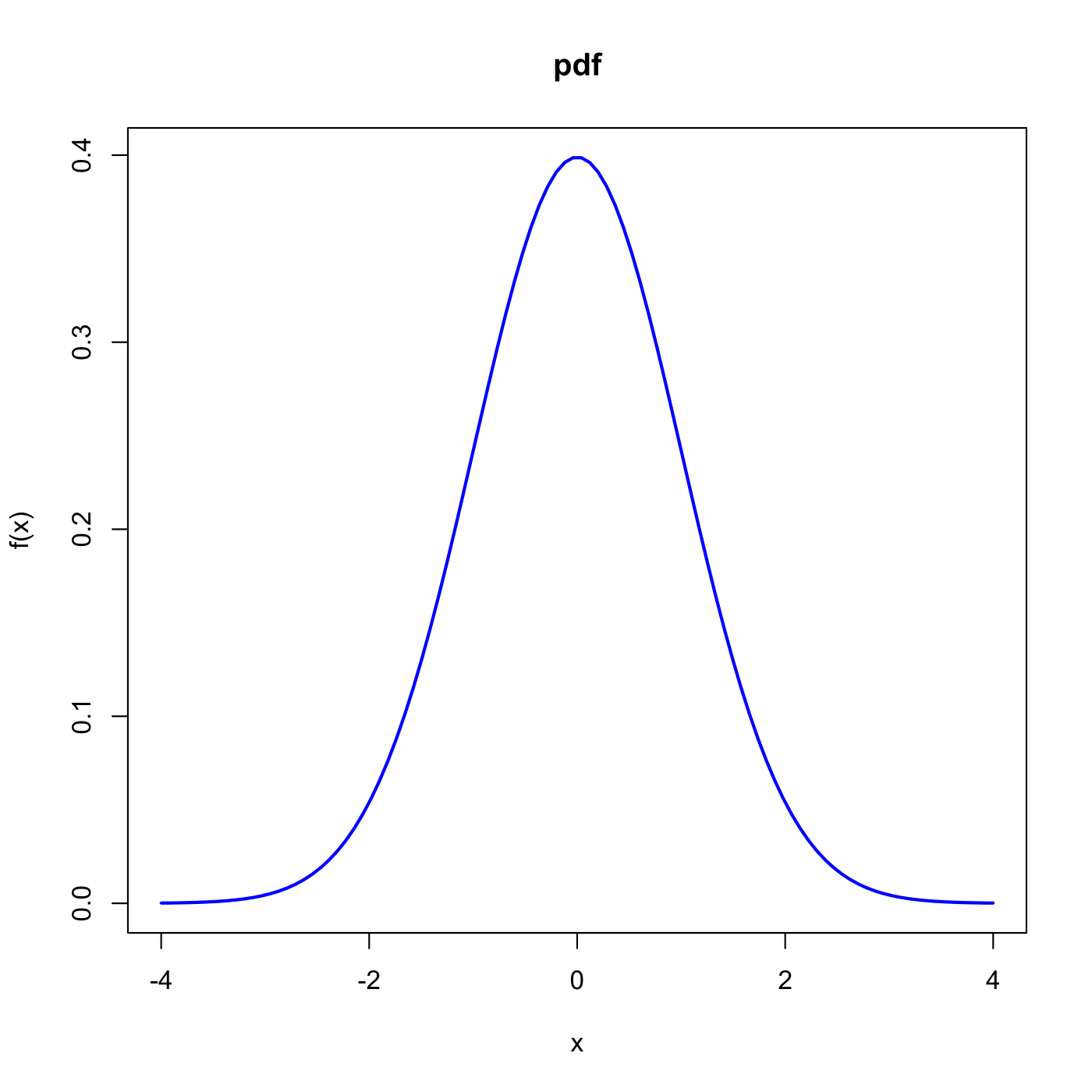
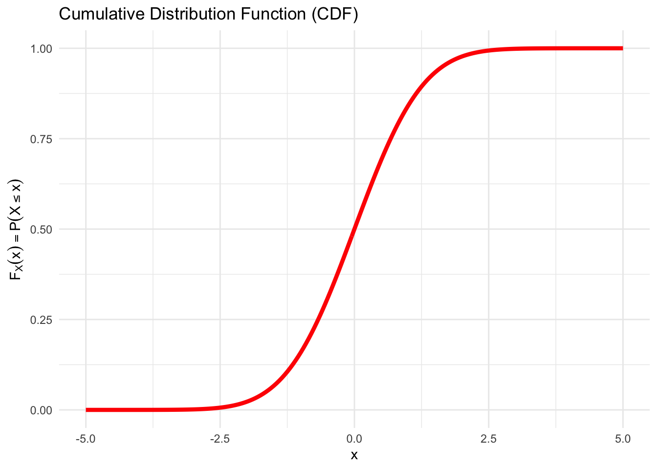
Figure 5.2: A typical bell-shaped Density Function

and a CDF that has the shape of an S.

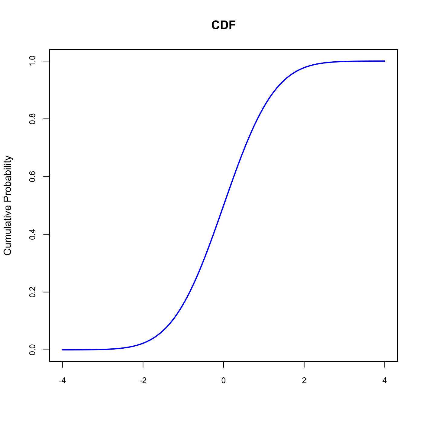
Figure 5.3: A typical S-shaped Cumulative Distribution Function

5.3 Distributional Summaries

5.3.1 The Expectation

Recall that for Discrete random variables, the Expectation results from summing the product of \(x_{i}\) and \(p_{i}=P(X=x_{i})\), for all possible values \(x_{i}\)

\[\begin{equation*} E\left[ X\right] =\sum_{i}x_{i}p_{i} \end{equation*}\]

5.3.2 The Variance

Recall that, for discrete random variables, we defined the variance as:

\[\begin{equation*} Var\left( X\right) =\sum_{i}\left( x_{i}-E\left[ X\right] \right) ^{2}P \left( X=x_{i}\right) \end{equation*}\]

Very roughly speaking, we could say that we are replacing the sum (\(\sum\)) by its continuous counterpart, namely the integral (\(\int\)).

5.3.3 Important properties of expectations

As with discrete random variables, the following properties hold when \(X\) is a continuous random variable and \(c\) is any real number (namely, \(c \in \mathbb{R}\)):

• \(E\left[ cX\right] =cE\left[ X\right]\)
• \(E\left[ c+X\right] =c+E\left[ X\right]\)
• \(Var\left( cX\right) =c^{2}Var\left( X\right)\)
• \(Var\left( c+X\right) =Var\left( X\right)\)

Let us consider, for instance, the following proofs for first two properties. To compute \(E\left[ cX\right]\) we take advantage of the linearity of the integral with respect to multiplication by a constant. \[\begin{eqnarray*} E\left[ cX\right] &=&\int \left( cx\right) f_{X}\left( x\right) dx \\ &=&c\int xf_{X}\left( x\right) dx \\ &=&cE\left[ X\right]. \end{eqnarray*}\]

In the same way, to evaluate \(E\left[ c+X\right]\), we take advantage of the linearity of integration and of the fact that \(f(x)\) is a density and integrates to 1 over the whole domain of integration. \[\begin{eqnarray*} E\left[ c+X\right] &=&\int \left( c+x\right) f_{X}\left( x\right) dx \\ &=&\int cf_{X}\left( x\right) dx+\int xf_{X}\left( x\right) dx \\ &=&c\times 1+E\left[ X\right] \\ &=&c+E\left[ X\right]. \end{eqnarray*}\]

5.3.4 Mode and Median

There are two other important distributional summaries that also characterise a sort of center for the distribution: the Mode and the Median.

The Mode of a continuous random variable having density \(f_{X}(x)\) is the value of \(x\) for which the PDF \(f_X(x)\) attains its maximum, i.e.\[\text{Mode}(X) = \text{argmax}_{x}\{f_X(x)\}.\] Very roughly speaking, it is the point with the highest concentration of probability.

On the other hand, the Median of a continuous random variable having CDF \(F_{X}(x)\) is the value \(m\) such that \(F(m) = 1/2\) \[\text{Median}(X) = \text{arg}_{m}\left\{P(X\leq m) = F_X(m) = \frac{1}{2}\right\}.\] Again, very roughly speaking, the median is the value that splits the sample space in two intervals with equal cumulative probability.

Let’s illustrate these two location values in the PDF. We have purposefully chosen an asymmetric (right)skewed distribution to display the differences between these two values.

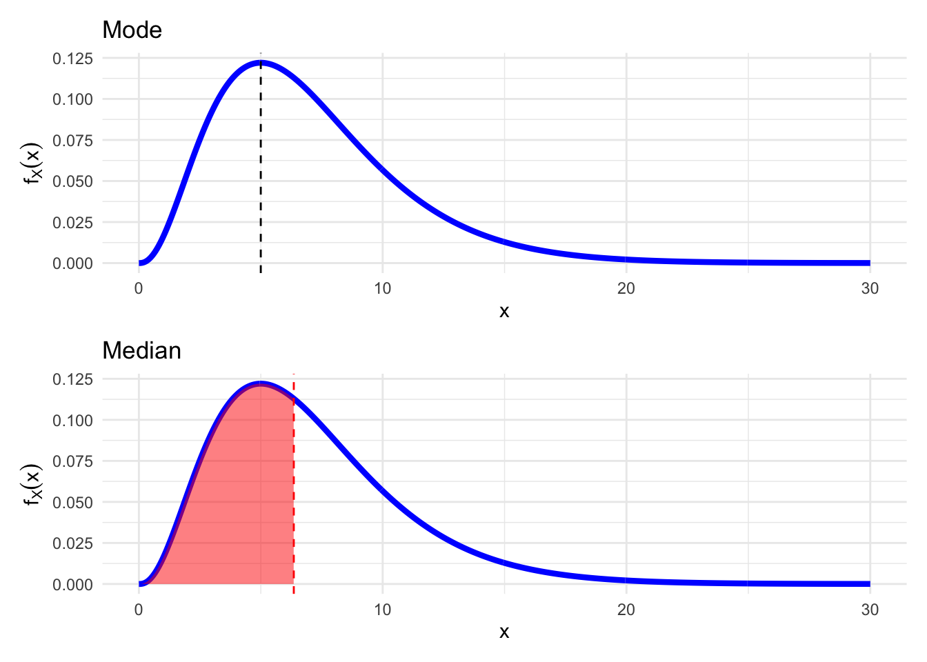
Figure 5.4: Mode and Median of an asymmetric distribution

5.4 Some Important Continuous Distributions

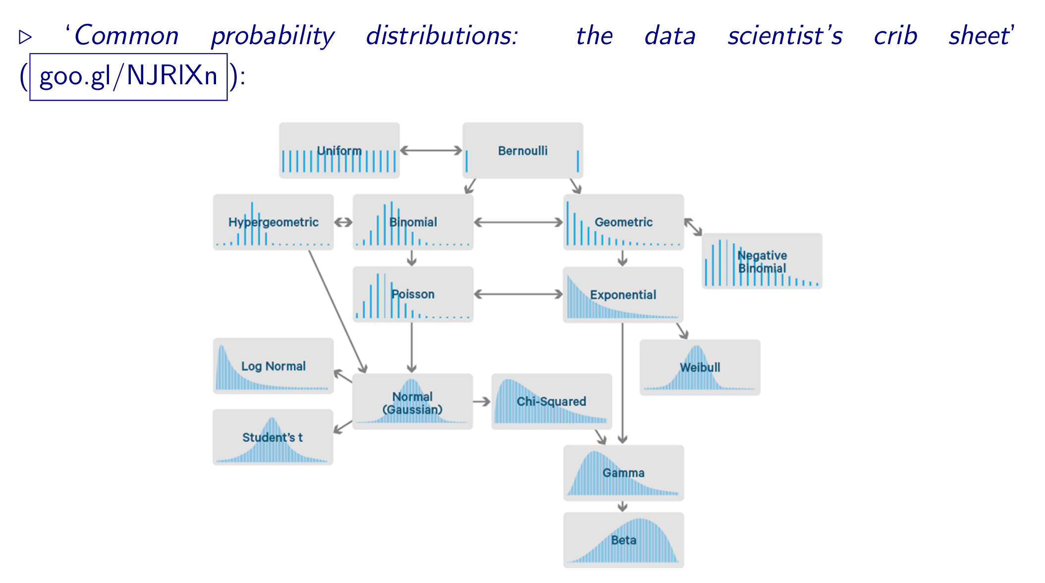
There is a wide variety of Probability Distributions. In this section, we will explore the properties of some of them, namely:

• Continuous Uniform
• Gaussian a.k.a. “Normal”
• Chi-squared
• Student’s \(t\)
• Fisher’s \(F\)
• Log-Normal
• Exponential

5.4.1 Continuous Uniform Distribution

As a graphical illustration, let us consider the case when \(a=0\) and \(b=1\). So, we have that the density is 1 on the interval \((0,1)\) and 0 everywhere else: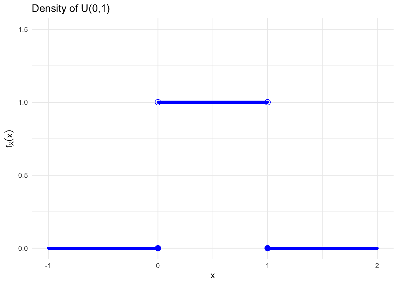

Figure 5.5: Density of a Continuous Uniform Random Variable

5.4.1.1 Expectation

The expected value of \(X\) can be computed via integration: \[\begin{eqnarray*} E\left[ X\right] &=&\int_{a}^{b}\frac{x}{\left( b-a\right) }dx \\ &=&\frac{1}{\left( b-a\right)} \int_{a}^{b} x dx \\ &=& \frac{1}{\left( b-a\right)} \left[\frac{x^{2}}{2}\right] _{a}^{b} \\ &=&\frac{1}{\left(b-a\right)}\left[\frac{b^{2}}{2}-\frac{a^{2}}{2}\right]\\ &=&\frac{1}{2\left(b-a\right)}\left[(b-a)(b+a)\right]\\ &=&\frac{a+b}{2} \end{eqnarray*}\]

5.4.1.2 Variance

By definition, the variance of \(X\) is given by: \[\begin{eqnarray*} Var\left( X\right) &=&\int_{a}^{b}\left[] x-\left( \frac{a+b}{2}\right) \right]^{2}\frac{1}{b-a}dx \\ &=&E\left[ X^{2}\right] -E\left[ X\right] ^{2} \end{eqnarray*}\]

Since we know the values of the second term: \[\begin{equation*} E\left[ X\right] ^{2}=\left( \frac{a+b}{2}\right) ^{2}, \end{equation*}\] we only need to work out the first term, i.e.  \[\begin{eqnarray*} E\left[ X^{2}\right] &=&\int_{a}^{b}\frac{x^{2}}{b-a}dx =\left. \frac{x^{3}}{3\left( b-a\right) }\right\vert _{a}^{b} \\ &=&\frac{b^{3}-a^{3}}{3\left( b-a\right) } = \frac{(b-a)\left( ab+a^{2}+b^{2}\right)}{3\left( b-a\right) } \\ &=&\frac{\left( ab+a^{2}+b^{2}\right) }{3}. \end{eqnarray*}\]

Putting both terms together, we get that the variance of \(X\) is given by: \[\begin{eqnarray*} Var\left( X\right) &=&\frac{\left( ab+a^{2}+b^{2}\right) }{3}-\left( \frac{% a+b}{2}\right) ^{2} \\ &=&\frac{1}{12}\left( a-b\right) ^{2} \end{eqnarray*}\]

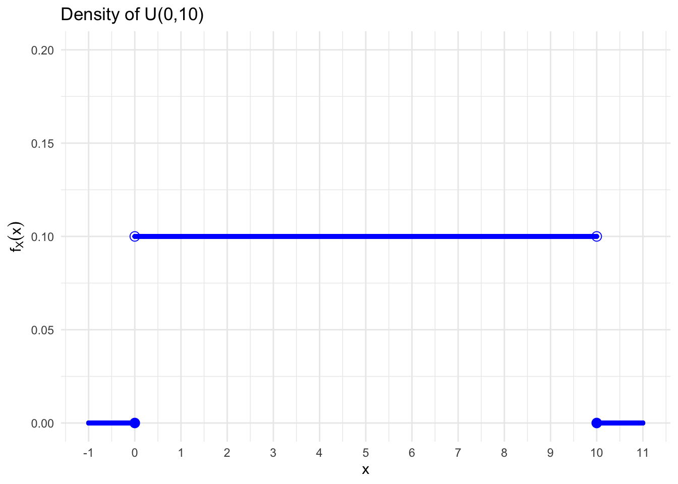
Figure 5.6: Density of \(X \sim \mathcal{U}(0,10)\)

We can compute the probabilities of different intervals: \[\begin{align} P(0\leq x \leq 1) &= \int_{0}^{1} 0.1x dx &= &0.1 x \left.\right\vert_{x=0}^{x=1} \\ &= 0.1\cdot(1-0) &= &0.1 \\ P(0\leq x \leq 2) &= 0.1\cdot (2-0) &= &0.2 \\ P(2\leq x \leq 4) &= P(2\leq x \leq 4) &= &0.2 \\ P(x \geq 2) &= P(2 < x \leq 10) &= &0.1(10-2) = 0.8 \end{align}\]

Let’s represent graphically the \(P(X\geq 2)\). Indeed, we see that it is represented by the pink rectangle. If we compute the area, it is apparent that its value is \(0.8\), as we have obtained with the formula.

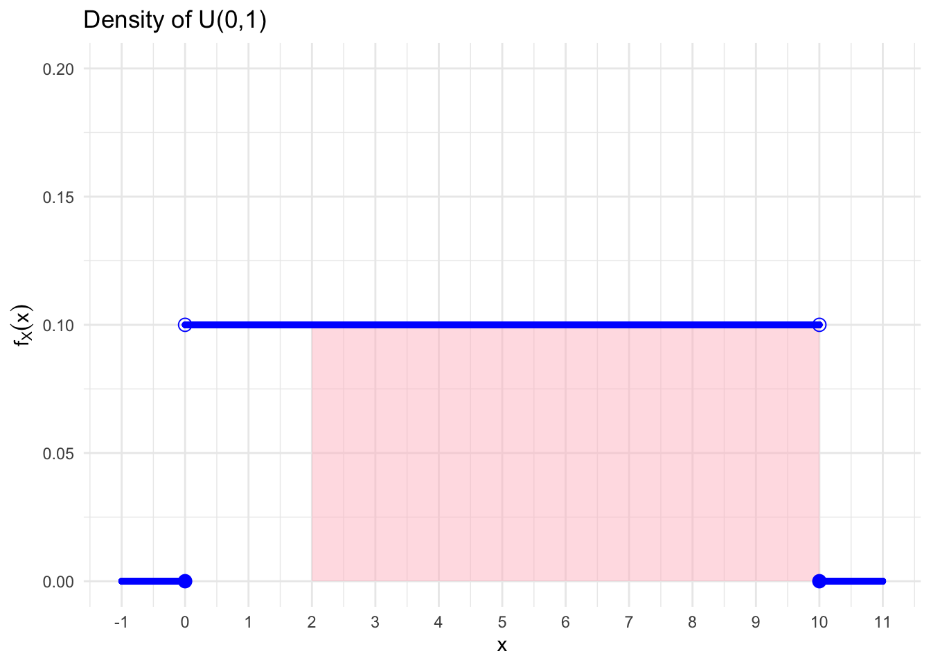
Figure 5.7: Cumulated Probability between 2 and 10

5.4.2 Normal (Gaussian) distribution

The Normal distribution was “discovered” in the eighteenth century when scientists observed an astonishing degree of regularity in the behavior of measurement errors.

They found that the patterns (distributions) that they observed, and which they attributed to chance, could be closely approximated by continuous curves which they christened the “normal curve of errors”.

The mathematical properties of these curves were first studied by:

• Abraham de Moivre (1667-1745),
• Pierre Laplace (1749-1827), and then
• Karl Gauss (1777-1855), who also lent his name to the distribution.

There are couple of important properties worth mentioning:

• A Normal random variable \(X\) can take any value \(x\in\mathbb{R}\).
• A Normal distribution is completely defined by its mean \(\mu\) and its variance \(\sigma ^{2}\). This means that infinitely many different normal distributions are obtained by varying the parameters \(\mu\) and \(\sigma ^{2}\).

To illustrate this last property, we plot a series of densities that result from replacing different values of \(\mu\) and \(\sigma^2\) in the following figure:

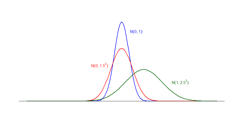
Figure 5.8: Densities for \(\color{blue}{X_{1}\sim\mathcal{N}(0,1)}\), \(\color{red}{X_{2}\sim\mathcal{N}(0,1.5^2)}\), \(\color{forestgreen}{X_{3}\sim\mathcal{N}(1,2.5^2)}\)

• As we can assess in the previous Figure ??, the PDF of the Normal Distribution is “Bell-shaped”, meaning that looks a little bit like a bell. Moreover, it is:
  • Symmetric, i.e. it is not skewed either to the right or to the left. This also implies that the values of the density are the same for \(x\) and \(-x\), i.e \(\phi_{(\mu,\sigma)}(x) = \phi_{(\mu,\sigma)}(-x)\)
  • Unimodal, meaning that it has only one mode and
  • The Mean, Median and Mode are all equal, owing to the symmetry of the distribution.

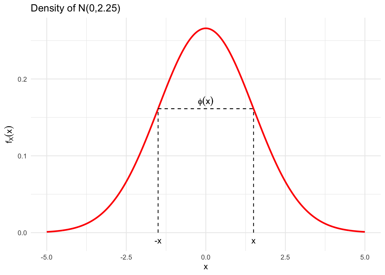
Figure 5.9: The symmetry of the Gaussian Distribution

5.4.2.1 The Standard Normal distribution

First let us establish that \(\phi_{(\mu,\sigma)}(x)\) can serve as a density function. To show that, we need to demonstrate that it integrates to 1 in all the domain \(\mathbb{R}\)

Integrating with respect to \(x\) using integration by substitution we obtain \[\begin{eqnarray*} \int_{-\infty}^{\infty}\phi_{(\mu,\sigma)}(x)dx&=& \int_{-\infty}^{\infty}\frac{1}{\sqrt{2\pi\sigma^2}}\exp{\left\{-\frac{(x-\mu)^2}{2\sigma^2}\right\}}dx \\ &=&\int_{-\infty}^{\infty}\frac{1}{\sqrt{2\pi}}\exp{\left\{-\frac{z^2}{2}\right\}}dz \quad \text{where: } z=\frac{x-\mu}{\sigma} \Leftrightarrow dz = \frac{dx}{\sigma}. \end{eqnarray*}\] But the second integral on the right hand side equals to: \[ \int_{-\infty}^{\infty}\exp{\left\{-\frac{z^2}{2}\right\}}dz = 2\underbrace{\int_0^{\infty}\exp{\left\{-\frac{z^2}{2}\right\}}dz}_{={\sqrt{2\pi}} \big/ {2}} = \sqrt{2\pi} \] which is a known result, known as the Gaussian Integral that cancels out with \(1/\sqrt{2\pi}\) yielding the integration to 1. Hence, the function \(\phi_{(\mu,\sigma)}(x)\) does indeed define the PDF of a random variable with a mean \(\mu\) and a variance of \(\sigma^2\)

In shorthand notation, we can characterise this transformation in the following way. \[X\sim \mathcal{N}\left( \mu ,\sigma ^{2}\right)\Leftrightarrow Z=\frac{\left( X-\mu \right) }{\sigma }\sim \mathcal{N}\left( 0,1\right)\] This process of standardisation has very important implications when dealing with the Normal Distribution, one of them being the that one can compute all quantities related with a random variable \(X\) by evaluating the related quantities over \(Z\). This is an example of what is called called a variable transformation

In particular, we can transform from \(X\) to \(Z\) by “shifting” and “re-scaling”: \[\begin{equation*} Z=\frac{X-\mu }{\sigma } \ (\text{for the random variable}) \quad\mbox{and}\quad z=\frac{x-\mu }{\sigma }\, \ (\text{for its values}) , \end{equation*}\] and return back to \(X\) by a “re-scaling” and “shifting”: \[\begin{equation*} X=\sigma Z+\mu \ (\text{for the random variable}) \quad\mbox{and}\quad x=\sigma z+\mu\, \ (\text{for its values}) . \end{equation*}\]

Thus, statements about any Normal random variable can always be translated into equivalent statements about a standard Normal random variable, and viceversa.

5.4.2.2 The Normal CDF

For instance, we can concentrate on the consequences of this property on the computation of the CDF.

Analytically the CDF of a Normal Random Variable \(X\sim \mathcal{N}\left( \mu ,\sigma ^{2}\right)\) is given by:
\[\Phi_{(\mu,\sigma)}\left( x\right) =\int_{-\infty }^{x}\frac{1}{\sqrt{2\pi \sigma ^{2}}}\exp{ \left\{ -\frac{1}{2\sigma ^{2}}\left( t-\mu \right) ^{2}\right\}} dt\] To calculate \(\Phi_{(\mu,\sigma)}\left( x\right)=P(\{X\leq x\})\) we use integration with the substitution \(s=(t-\mu)/\sigma\), which implies: \(z=(x-\mu)/\sigma\) (for the domain of integration) and \(ds=dt/\sigma\) (for the “differential”), yielding: \[\begin{eqnarray*} P(\{ X\leq x\} )&=&\int_{-\infty}^x\frac{1}{\sqrt{2\pi\sigma^2}}\exp{\left\{-\frac{(t-\mu)^2}{2\sigma^2}\right\}}dt\\ &=&\int_{-\infty}^z\phi(s)ds\\ P(\{ X\leq x\} ) &=&P(\{Z\leq z\}) \end{eqnarray*}\]

Hence, the probability of the interval \(X\leq x\) has been mapped into a corresponding probability for a standard Normal random variable. In other words:

\[P(\{ X\leq x\}) = P\left(\left\{\underbrace{\frac{X-\mu}{\sigma}}_Z\leq \underbrace{\frac{x-\mu}{\sigma}}_{z}\right\}\right) = P(\{ Z\leq z\})\]

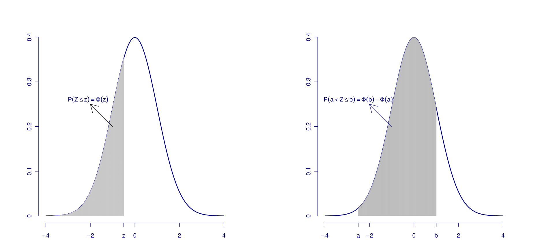
The integral that defines the CDF of a Standard Normal random variable: \[P(\{Z\leq z\})=\Phi(z)=\int_{-\infty}^z\phi(s)ds\] does not have a closed-form expression. Yet, it is possible to provide very precise numerical approximations using computers. Some of these values can be found in so-called Standard Normal Tables, which contain values of the integral \(\Phi(z)\) for various values of \(z\geq 0\).

To compute the cumulative probability for \(z\leq 0\) we take advantage of the symmetry property of \(\phi(z)\) i.e. \(\phi(z)=\phi(-z)\), which also implies that: \[\Phi(-z)=1-\Phi(z)\,\]

We can see this in the following plot.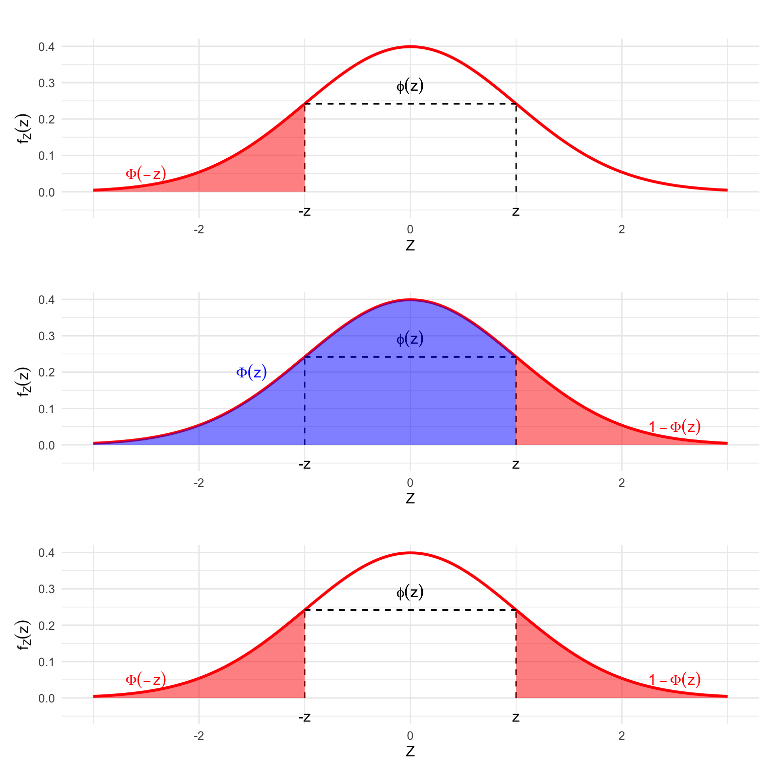

Figure 5.10: The Symmetry of the Standard Normal PDF and its consequences for the CDF

To compute the probability in a closed interval, if \(X\sim \mathcal{N}\left( \mu ,\sigma ^{2}\right)\) we can proceed by substraction: \[\begin{eqnarray*} P(\{x_1<X\leq x_2\})&=&P(\{z_1<Z\leq z_2\})\\ &=&P(\{Z\leq z_2\}) - P(\{Z\leq z_1\})\\ &=&\Phi(z_2)-\Phi(z_1) \end{eqnarray*}\] where, again, the values \(z_1\) and \(z_2\) result from standardisation \(z_1=(x_1-\mu)/\sigma\) and \(z_2=(x_2-\mu)/\sigma\). As we can see from the plot below, there’s a clear geometric interpretation to this relation.

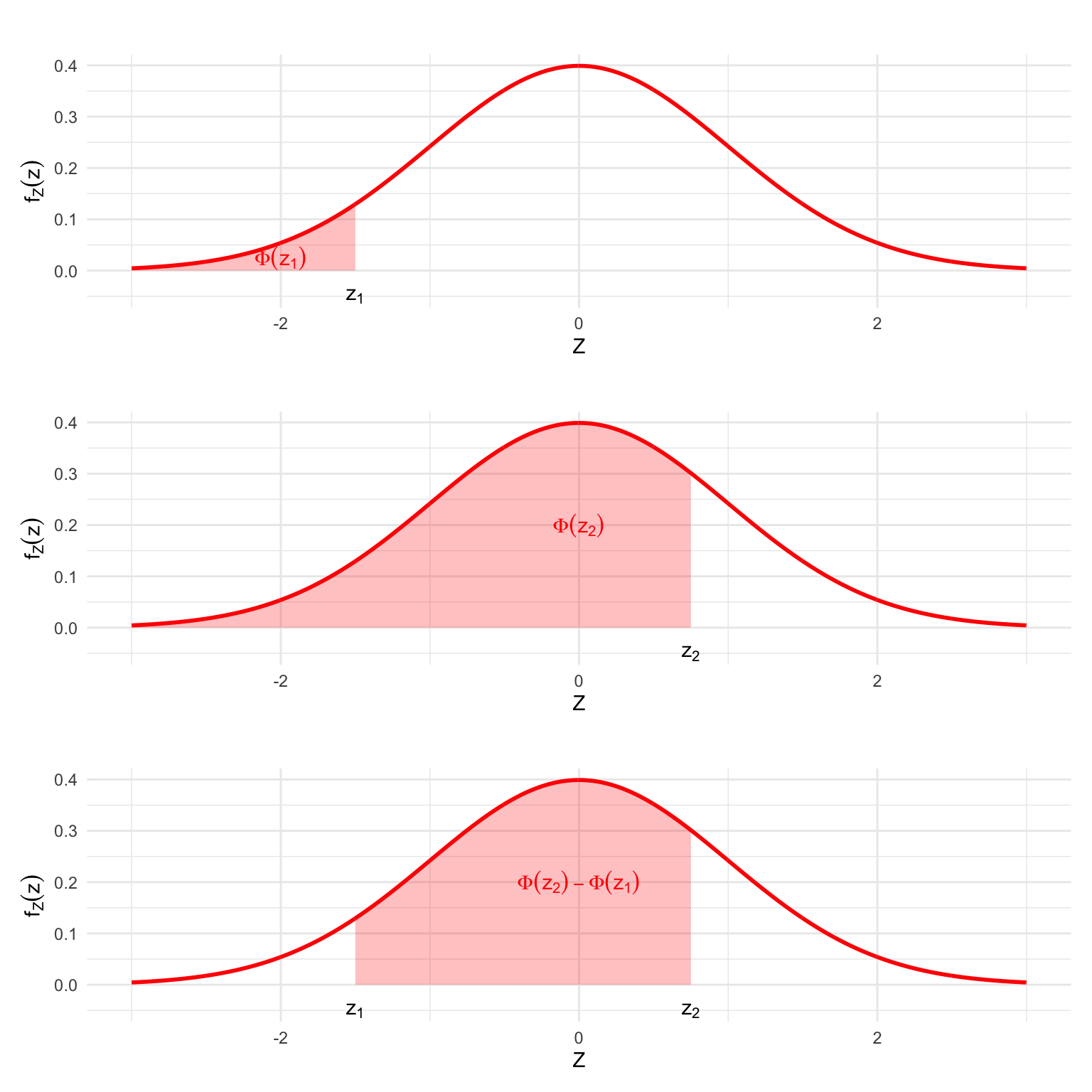
Figure 5.11: Computing the Probability of an interval

5.4.2.3 Standard Normal Tables

Standard Normal Tables give values of the standard normal integral \(\Phi(z)\) for \(z\geq 0\). This is done to , to save space, since values for negative \(z\) are obtained via symmetry, as we mentioned in the previous section.

Most of the tables are explicit in this choice and graphically show that they contain the probabilities of the interval \(0\leq Z \leq z\), e.g.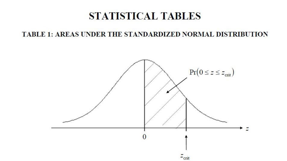 

Figure 5.12: Description of the contents of a Standard Normal Table

Typically, the dimension of the rows is nearest tenth to \(z\), while the columns indicate the nearest hundreth.

Say we would like to find the value of \(\Phi(0.46)\). We’d have to find the row for \(0.4\) and the column for 0.06.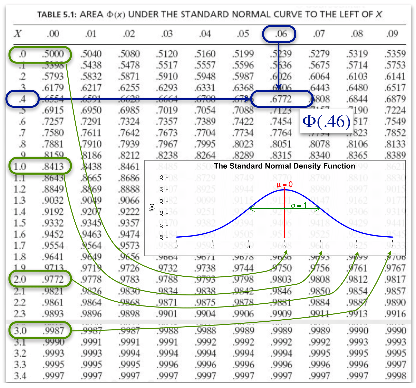

Figure 5.13: Probabilities for some values in the Standard Normal Table

You can use these tables to compute integrals/probabilities of intervals \(Z<=z\) or \(Z \in [z_1, z_2]\) using the rules mentioned above.

5.4.2.4 Further properties of the Normal distribution

The Rule ‘68 – 95 – 99.7’

In the following plot, the shaded areas under the PDFs are (approximately) equivalent to \(0.683\), \(0.954\) and \(0.997\), respectively.

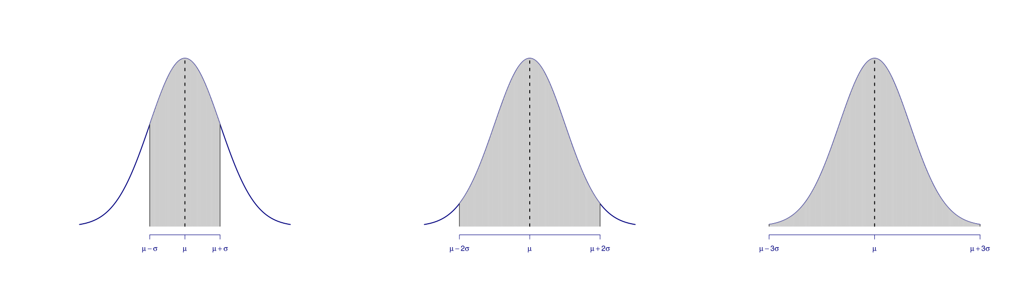
This leads to the rule: .’68 – 95 – 99.7’ i.e. that if \(X\) is a Normal random variable, \(X \sim \mathcal{N}(\mu, \sigma^2)\), its realization has approximately a probability of:

Probability	Interval
\(68 \, \%\)	\(\lbrack \mu - \sigma, \, \mu + \sigma \rbrack\)
\(95 \, \%\)	\(\lbrack \mu - 2 \, \sigma, \, \mu + 2 \, \sigma \rbrack\)
\(99.7 \, \%\)	\(\lbrack \mu - 3 \, \sigma, \, \mu + 3 \, \sigma\rbrack\)

• For \(X\sim \mathcal{N}\left( \mu ,\sigma ^{2}\right)\) \[\begin{equation*} E\left[ X\right] =\mu \text{ and }Var\left( X\right) =\sigma ^{2}. \end{equation*}\]

• If \(a\) is a number, then \[\begin{eqnarray*} X+a &\sim &\mathcal{N}\left( \mu +a,\sigma ^{2}\right) \\ aX &\sim &\mathcal{N}\left( a\mu ,a^{2}\sigma ^{2}\right). \end{eqnarray*}\]

• If \(X\sim \mathcal{N}\left( \mu ,\sigma ^{2}\right)\) and \(Y\sim \mathcal{N}\left( \alpha,\delta ^{2}\right)\), and \(X\) and \(Y\) are independent then \[\begin{equation*} X+Y\sim \mathcal{N}\left( \mu +\alpha ,\sigma ^{2}+\delta ^{2}\right). \end{equation*}\]

To illustrate the last point, let’s use simulated values for two independent normally-distributed random variables \(X\sim \mathcal{N}(5,1)\) and \(Y\sim \mathcal{N}(7,1)\), alongside their sum.

We can see that if we plot the densities of these RV’s independently, we have the expected normal density (two bell-shaped curves centered around 5 and 7 that are similar in shape since they sport the same variance). Moreover the density of the sum of the simulated values is also bell-shaped and appears to be centered around 12 and sports a wider variance, confirming visually what we expected, i.e. that \(X + Y \sim \mathcal{N}(5+7,1+1)\), \(X+Y \sim \mathcal{N}(12,2)\).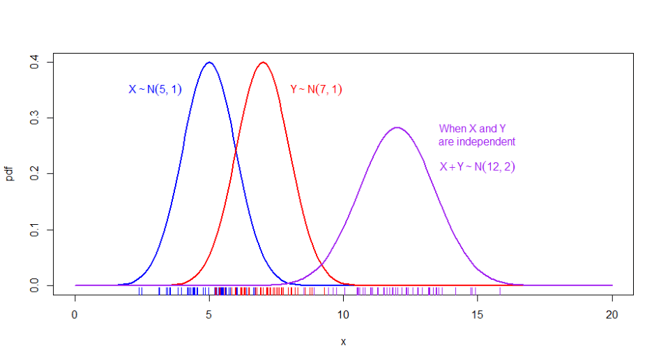

Figure 5.14: Locations of \(n=30\) sampled values of \(X,\) \(Y\), and \(X+Y\) shown as tick marks under each respective density

5.4.2.5 An example

5.4.3 The Chi-squared distribution

A Chi-Squared-distributed Random Variable has the following properties:

• \(X\sim \chi ^{2}(n)\) can take only positive values.
• The expectation and variance for \(X\sim \chi ^{2}(n)\), are given by: \[\begin{eqnarray*} E\left[ X\right] &=&n \\ Var\left( X\right) &=&2n \end{eqnarray*}\]
• Finally, if \(X\sim \chi ^{2}(n)\) and \(Y\sim \chi ^{2}(m)\) are independent then \(X+Y\sim \chi ^{2}(n+m)\).

The Chi-Squared distribution has a parameter that defines its shape, namely the \(n\) degrees of freedom. To illustrate their effect, let’s plot some densities in the following plot.

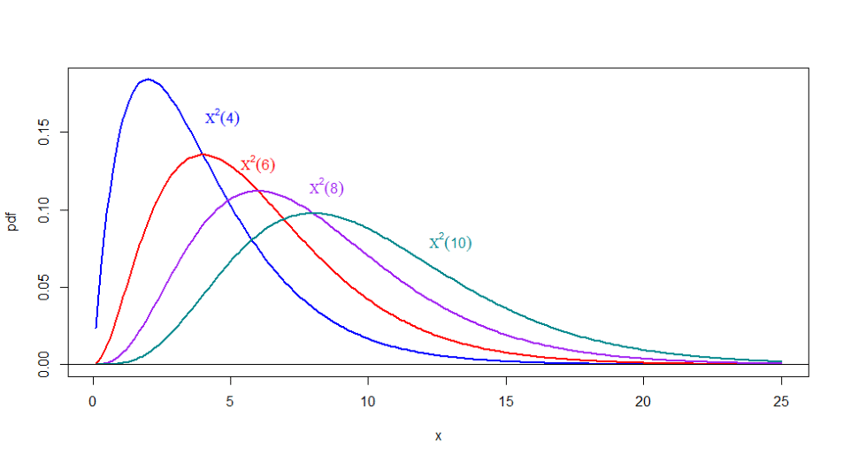
Figure 5.15: Chi-Squared densities for various values of \(n\)

5.4.3.1 Chi-squared tables

As you can imagine, cumulated probabilities for Chi-squared distributions are not straightforward to compute. To do it, we require computational methods.

Given that the shape depends on the parameter \(n\) there would be an infinite number of tables (as many as \(n\)) should we want to carry along the values of the CDF. Instead, tables contain the values for the Upper-tail or Lower-tail Quantiles for some given probabilities. For instance, in the following plot, we have a typical table, containing the values of the quantiles for different upper-tail probabilities displayed according to the degrees of freedom (denoted as \(V\)).

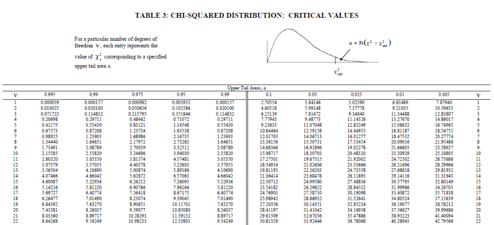
Figure 5.16: A typical Chi-square Table

5.4.4 The Student-t distribution

• \(T\sim t_{v}\,\) can take any value in \(\mathbb{R}\).
• Expected value and variance for \(T\sim t_{v}\) are \[\begin{eqnarray*} E\left[ T\right] &=&0\text{, for }v>1 \\ Var\left( T\right) &=&\frac{v}{v-2}\text{, for }v>2. \end{eqnarray*}\]

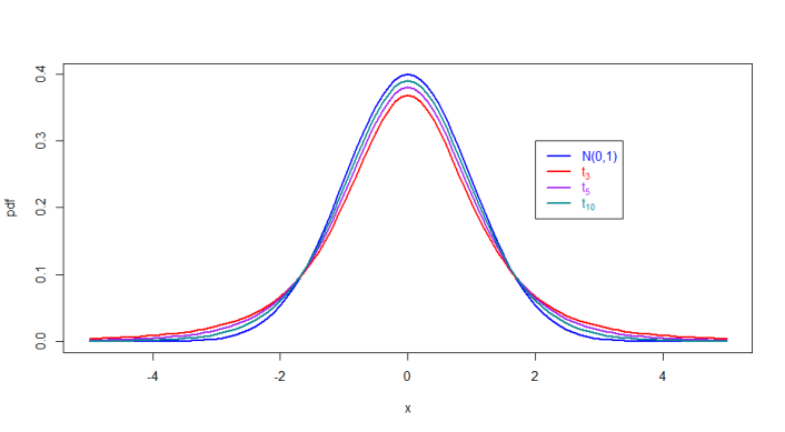
Figure 5.17: Densities for various Student-t densities alongside the Normal Density

Again, since the distribution depends on the degrees of freedom \(v\), in the absence of computers, we rely on tables for some values of upper-tail probabilities.

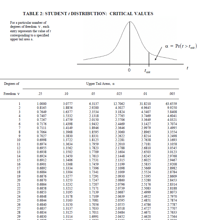
Figure 5.18: A typical Student’s-t Table

5.4.5 The F distribution

• \(F\sim F_{v_{1},v_{2}}\,\) can take only positive values.
• Expected value and variance for \(F\sim F_{v_{1},v_{2}}\) (note that the order of the degrees of freedom is important!) is given by: \[\begin{eqnarray*} E\left[ F\right] &=&\frac{v_{2}}{v_{2}-2}\text{, for }v_{2}>2 \\ Var\left( F\right) &=&\frac{2v_{2}^{2}\left( v_{1}+v_{2}-2\right) }{% v_{1}\left( v_{2}-2\right) ^{2}\left( v_{2}-4\right) }\text{, for }v_{2}>4. \end{eqnarray*}\]

As we can assess from the following plot, there is no uniform way in which the densities change according to the degrees of freedom. However all of them seem to be concentrated towards the lower side of the \(\mathbb{R}^{+}\) line.

Again, when distributed in tables, we can only obtain information on the quantiles for some upper-tail probabilites. However, since the distributions are defined by two sets of degrees of freedom, a table can only pertain one value of the upper tail probability.

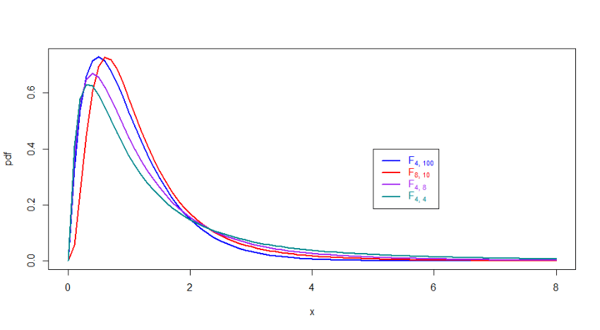
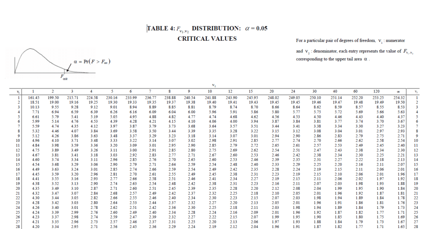
Figure 5.19: Critical Values for \(F\) distribution and \(\alpha = 0.05\)

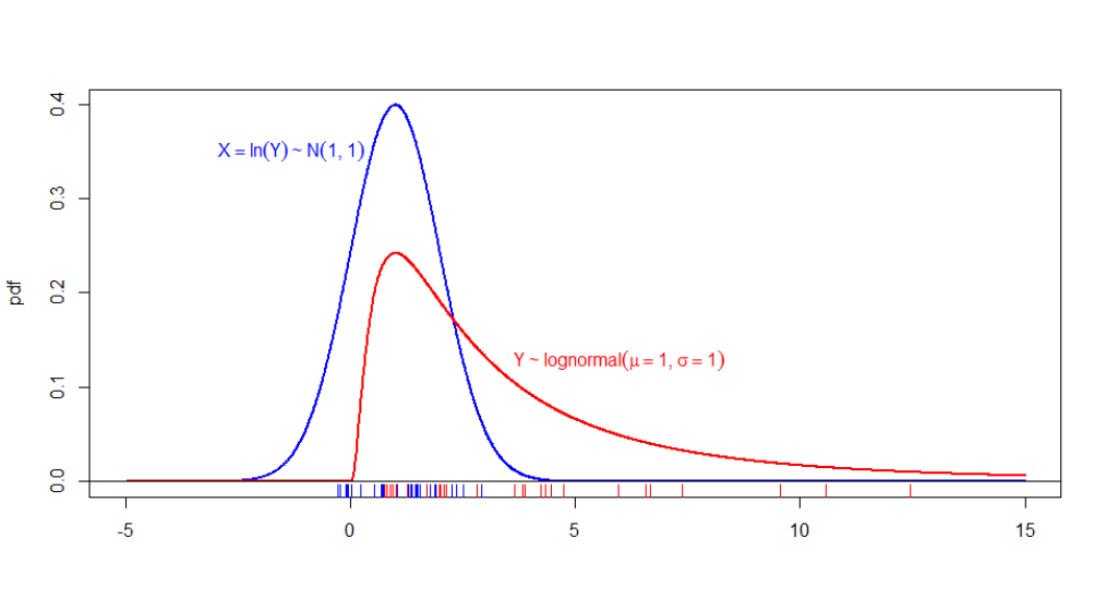
5.4.6 The lognormal distribution

• If \(Y\sim\) \(\left( \mu ,\sigma ^{2}\right)\) then \[\begin{eqnarray*} E\left[ Y\right] &=&\exp^{ \left( \mu +\frac{1}{2}\sigma ^{2}\right)} \\ Var(Y) &=&\exp^{ \left( 2\mu +\sigma ^{2}\right)} \left( \exp^{ \left( \sigma ^{2}\right)} -1\right). \end{eqnarray*}\]

In the next plot, we display an estimation of the density of the realization of a Normal Random Variable, as well as the density of \(y = exp(x)\). Notice how the distribution is assymetric, positive and right-skewed.

5.4.7 Exponential distribution

• The Expectation and Variance of \(X\sim \text{Exp}(\lambda)\) are as follows:

\[\begin{eqnarray*} E[X]=\int_{0}^{\infty }xf_X(x )dx= 1/\lambda & \text{and} & Var(X)=\int_{0}^{\infty }x^{2}f_X(x )dx-E^{2}(X)=1/\lambda ^{2}. \nn \end{eqnarray*}\]

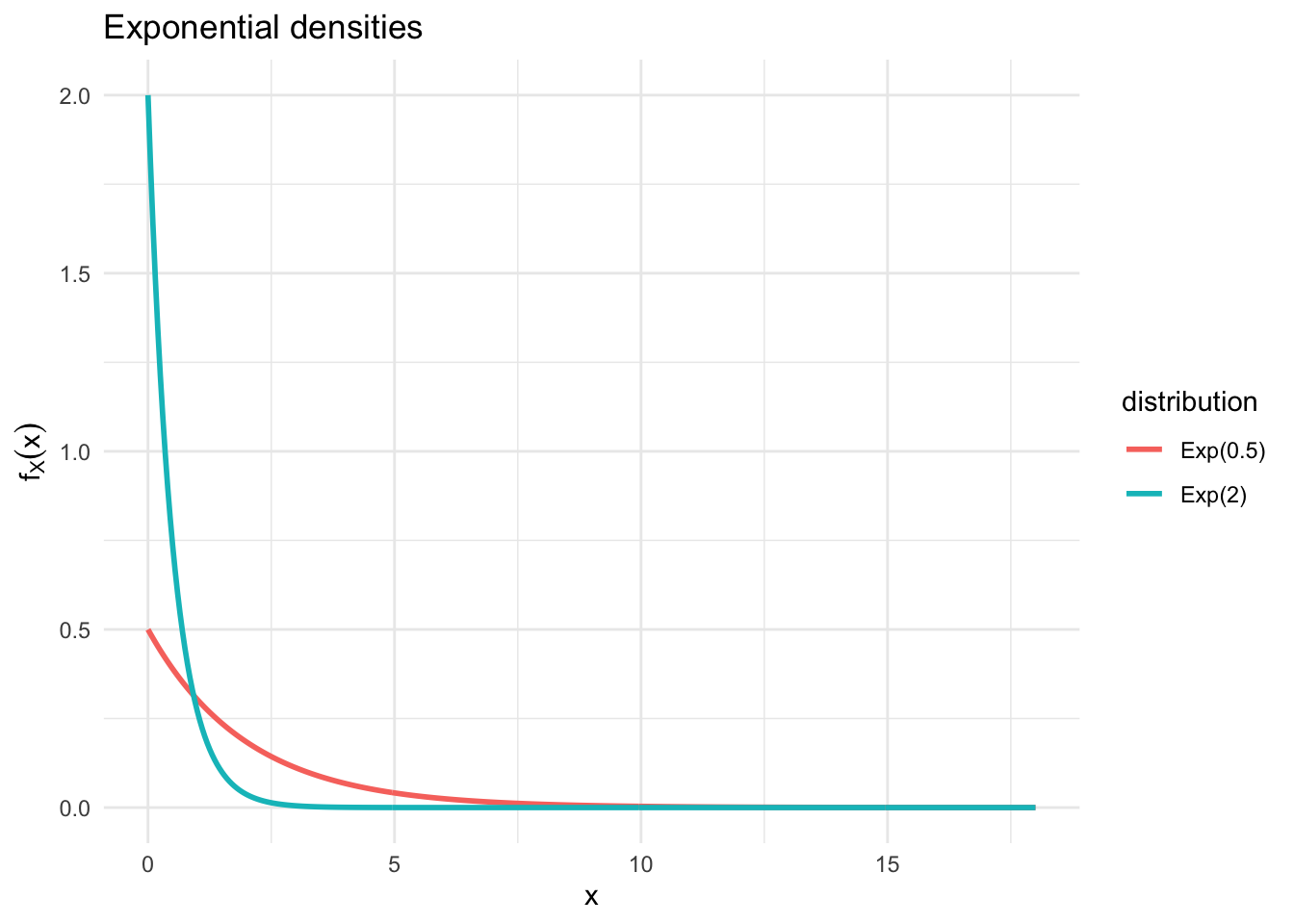
Figure 5.20: Graphical Illustration of Exponential distributions with varying \(\lambda\)

5.5 Transformation of variables

• Consider a random variable \(X\)
• Suppose we are interested in \(Y=\psi(X)\), where \(\psi\) is a one to one function
• A function \(\psi \left( x\right)\) is one to one (1-to-1) if there are no two numbers, \(x_{1},x_{2}\) in the domain of \(\psi\) such that \(\psi \left( x_{1}\right) =\psi \left( x_{2}\right)\) but \(x_{1}\neq x_{2}\).
• A sufficient condition for \(\psi \left( x\right)\) to be 1-to-1 is that it be monotonically increasing (or decreasing) in \(x\).
• Note that the inverse of a 1-to-1 function \(y=\psi \left(x\right)\) is a 1-to-1 function \(\psi^{-1}\left( y\right)\) such that:

\[\begin{equation*} \psi ^{-1}\left( \psi \left( x\right) \right) =x\text{ and }\psi \left( \psi ^{-1}\left( y\right) \right) =y. \end{equation*}\]

• To transform \(X\) to \(Y\), we need to consider all the values \(x\) that \(% X\) can take
• We first transform \(x\) into values \(y=\psi (x)\)

5.5.1 Transformation of discrete random variables

• To transform a discrete random variable \(X\), into the random variable \(Y=\psi (X)\), we transfer the probabilities for each \(x\) to the values $y=( x) $:

\(X\)	\(P \left(\{ X=x_{i} \}\right) =p_{i}\)		\(Y\)	\(P \left(\{X=x_{i} \}\right) =p_{i}\)
\(x_{1}\)	\(p_{1}\)	\(\qquad \Rightarrow \qquad\)	\(\psi (x_{1})\)	\(p_{1}\)
\(x_{2}\)	\(p_{2}\)		\(\psi (x_{2})\)	\(p_{2}\)
\(x_{3}\)	\(p_{3}\)		\(\psi (x_{3})\)	\(p_{3}\)
\(\vdots\)	\(\vdots\)		\(\vdots\)	\(\vdots\)
\(x_{n}\)	\(p_{n}\)		\(\psi (x_{n})\)	\(p_{n}\)

Notice that this is equivalent to applying the function \(\psi \left(\cdot \right)\) inside the probability statements:

\[\begin{eqnarray*} P \left( \{ X=x_{i} \}\right) &=&P \left( \{\psi \left( X\right) =\psi \left( x_{i}\right) \} \right) \\ &=&P \left( \{ Y=y_{i} \} \right) \\ &=&p_{i} \end{eqnarray*}\]

Indeed, after two tosses, there are four possible coin sequences, \[ \{HH,HT,TH,TT\} \] although not all of them result in different stock prices at time \(t_2\).

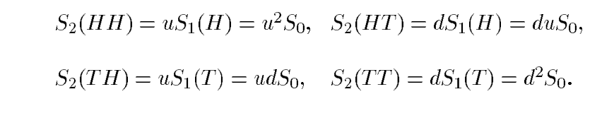
Let us set \(S_0=1\), \(u=2\) and \(d=1/2\): we represent the price evolution by a tree:

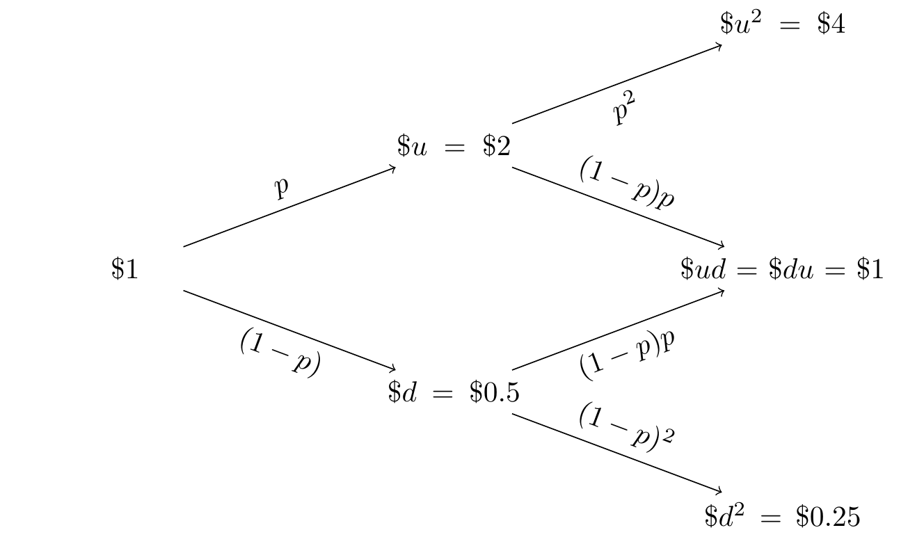
Now consider an European option call with maturity \(t_2\) and strike price \(K=0.5\), whose random pay-off at \(t_2\) is \(C=\max(0;S_2-0.5)\). Thus, \[\begin{eqnarray*} C(HH)=\max(0;4-0.5)=\$ 3.5 & C(HT)=\max(0;1-0.5)=\$ 0.5 \\ C(TH)=\max(0;1-0.5)=\$ 0.5 & C(TT)=\max(0;0.25-0.5)=\$ 0. \end{eqnarray*}\] Thus at maturity \(t_2\) we have

\(S_2\)	\(P \left(\{ X=x_{i} \}\right) =p_{i}\)		\(C\)	\(P \left(\{C=c_{i} \}\right) =p_{i}\)
\(\$ u^2\)	\(p^2\)	\(\qquad \Rightarrow \qquad\)	\(\$ 3.5\)	\(p^2\)
\(\$ ud\)	\(2p(1-p)\)		\(\$ 0.5\)	\(2p(1-p)\)
\(\$ d^2\)	\((1-p)^2\)		\(\$ 0\)	\((1-p)^2\)

Since \(ud=du\) the corresponding values of \(S_2\) and \(C\) can be aggregated, without loss of info.

5.5.2 Transformation of variables using the CDF

We can use the same logic for CDF probabilities, whether the random variables are discrete or continuous.

For instance, Let \(Y=\psi \left( X\right)\) with \(\psi \left( x\right)\) 1-to-1 and monotone increasing. Then:

\[\begin{eqnarray*} F_{Y}\left( y\right) &=&P \left( \{ Y\leq y \}\right) \\ &=&P \left( \{ \psi \left( X\right) \leq y \} \right) =P \left( \{ X\leq \psi ^{-1}\left( y\right) \} \right) \\ &=&F_{X}\left( \psi ^{-1}\left( y\right) \right) \end{eqnarray*}\]

You can notice that Monotone decreasing functions work in a similar way, but require changing of the sense of the inequality, e.g. let \(Y=\psi \left( X\right)\) with \(\psi \left( x\right)\) 1-to-1 and monotone decreasing. Then:

\[\begin{eqnarray*} F_{Y}\left( y\right) &=&P \left( \{ Y\leq y \} \right) \\ &=&P \left( \{ \psi \left( X\right) \leq y \} \right) =P \left( \{ X\geq \psi ^{-1}\left( y\right) \} \right) \\ &=&1-F_{X}\left( \psi ^{-1}\left( y\right) \right) \end{eqnarray*}\]

5.5.3 Transformation of continuous RV through PDF

For continuous random variables, if \(\psi \left( x\right)\) 1-to-1 and monotone increasing, we have: \[\begin{equation*} F_{Y}\left( y\right) =F_{X}\left( \psi ^{-1}\left( y\right) \right) \end{equation*}\] Notice this implies that the PDF of \(Y=\psi \left( X\right)\) must satisfy% \[\begin{eqnarray*} f_{Y}\left( y\right) &=&\frac{dF_{Y}\left( y\right) }{dy}=\frac{dF_{X}\left( \psi ^{-1}\left( y\right) \right) }{dy} \\ &=&\frac{dF_{X}\left( x\right) }{dx}\times \frac{d\psi ^{-1}\left( y\right) }{dy}\qquad \text{{\small (chain rule)}} \\ &=&f_{X}\left( x\right) \times \frac{d\psi ^{-1}\left( y\right) }{dy}\qquad \text{{\small (derivative of CDF (of }}X\text{){\small \ is PDF)}} \\ &=&f_{X}\left( \psi ^{-1}\left( y\right) \right) \times \frac{d\psi ^{-1}\left( y\right) }{dy}\qquad \text{{\small (substitute }}x=\psi ^{-1}\left( y\right) \text{{\small )}} \end{eqnarray*}\]

What happens when \(\psi \left( x\right)\) 1-to-1 and monotone decreasing? We have: \[\begin{equation*} F_{Y}\left( y\right) =1-F_{X}\left( \psi ^{-1}\left( y\right) \right) \end{equation*}\] So now the PDF of \(Y=\phi \left( X\right)\) must satisfy: \[\begin{eqnarray*} f_{Y}\left( y\right) &=&\frac{dF_{Y}\left( y\right) }{dy}=-\frac{% dF_{X}\left( \psi ^{-1}\left( y\right) \right) }{dy} \\ &=&-f_{X}\left( \psi ^{-1}\left( y\right) \right) \times \frac{d\psi ^{-1}\left( y\right) }{dy}\qquad \text{{\small (same reasons as before)}} \end{eqnarray*}\]

but \(\frac{d\psi ^{-1}\left( y\right) }{dy}<0\) since here \(\psi \left(\cdot \right)\) is monotone decreasing, hence we can write: \[\begin{equation*} f_{Y}\left( y\right) =f_{X}\left( \psi ^{-1}\left( y\right) \right) \times \left\vert \frac{d\psi ^{-1}\left( y\right) }{dy}\right\vert \end{equation*}\]

This expression (called Jacobian-formula) is valid for \(\psi \left( x\right)\) 1-to-1 and monotone (whether increasing or decreasing)

More generally, for \(\alpha\in[0,1]\), the \(\alpha\)-th quantile of a r.v. \(X\) is the value \(x_\alpha\) such that \(P(\{X \leq x_\alpha\})\geq\alpha\). If \(X\) si a continuous r.v. we can set \(P(\{X \leq x_\alpha\})=\alpha\) (as we did, e.g., for the lognormal).

5.5.4 A caveat

When \(X\) and \(Y\) are two random variables, we should pay attention to their transformations. For instance, let us consider \[ X\sim \mathcal{N}(\mu,\sigma^2) \quad \text{and} \quad Y\sim Exp(\lambda). \] Then, let’s transform \(X\) and \(Y\)

• in a linear way: \(Z=X+Y\). We know that \[ E[Z] = E[X+Y] = E[X] + E[Y] \] %so we can rely on the linearity of the expected value.
• in a nonlinear way \(W = X/Y\). One can show that

\[\color{red} E[W] = E\left[\frac{X}{Y}\right] \neq \frac{E[X]}{E[Y]}.\]

5.6 The big picture

Despite exotic names, the common distributions relate to each other in intuitive and interesting ways. Several follow naturally from the Bernoulli distribution, for example.