Chapter 3 Probability Axioms
Figure 3.1: ‘Is it clear to Everyone?’ by Enrico Chavez
In order to formalise probability as a branch of mathematics, Andrey Kolmogorov formulated a series of postulates. These axioms are crucial elements of the foundations on which all the mathematical theory of probability is built.
3.2 Properties of \(P(\cdot)\)
These three axioms are the building block of other, more sophisticated statements. For instance:

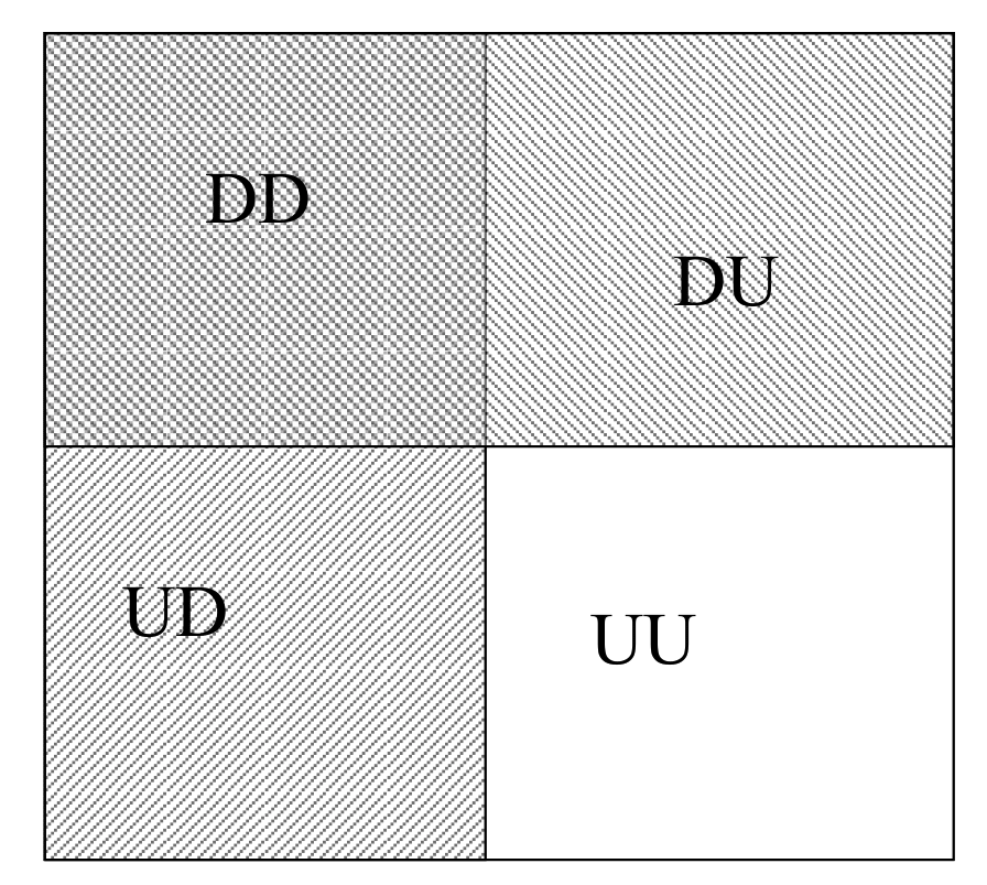
Figure 3.2: The areas of \(B\subset A\)
To illustrate this property, consider for instance \(n=2\). Then we have: \[ P(A_1 \cup A_2 ) = P(A_1) + P(A_2) - P(A_1 \cap A_2) \leq P(A_1) + P(A_2) \] since \(P(A_1 \cap A_2) \geq 0\) by definition.
3.4 Conditional probability
](img/fun/probconditionnelle2.png)
Figure 3.4: ‘Probability of a walk’ from the Cartoon Guide to Statistics
As a measure of uncertainty, the probability depends on the information available. The notion of Conditional Probability captures the fact that in some scenarios, the probability of an event will change according to the realisation of another event.
Let us illustrate this with an example:
Now let us define the event \(A\) = getting \(5\), or equivalently \(A=\{ 5\}\). What is \(P(A)\), i.e. the probability of getting \(5\)?. In the table above, we can identify and highlight the scenarios where the sum of both dice is 5:
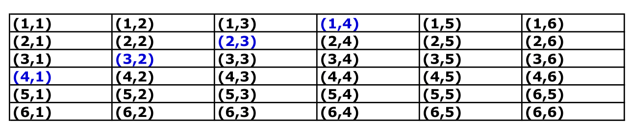
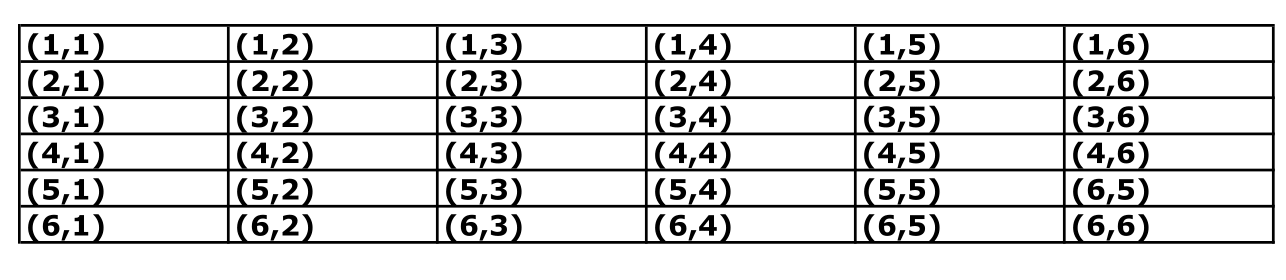
Since both dice are fair, we get 36 mutually exclusive scenarios with equal probability \({1}/{36}\), i.e. \[Pr(i,j) = \frac{1}{36}, \quad \text{for} \quad i,j=1,..,6\] Hence, to compute the probability of \(A\), we can sum their probability of the highlighted events: \[\begin{eqnarray} P(5) &=& Pr\left\{ (1,4) \cup (2,3) \cup (3,2) \cup (4,1) \right\} \\ &=& Pr\left\{ (1,4) \right\} + Pr\left\{ (2,3) \right\} + Pr\left\{(3,2) \right\} + Pr\left\{ (4,1) \right\} \\ &=& {1} /{36} + {1} /{36} + {1} /{36} + {1} /{36} \\ &=& {4} /{36} \\ &=& 1 /{9}. \end{eqnarray}\]
Now, suppose that, instead of throwing both dice simultaneously, we throw them one at a time. In this scenario, imagine that our first die yields a 2.
What is the probability of getting 5 given that we have gotten 2 in the first throw?
To answer this question, let us highlight the outcomes where the first die yields a 2 in the table of events.
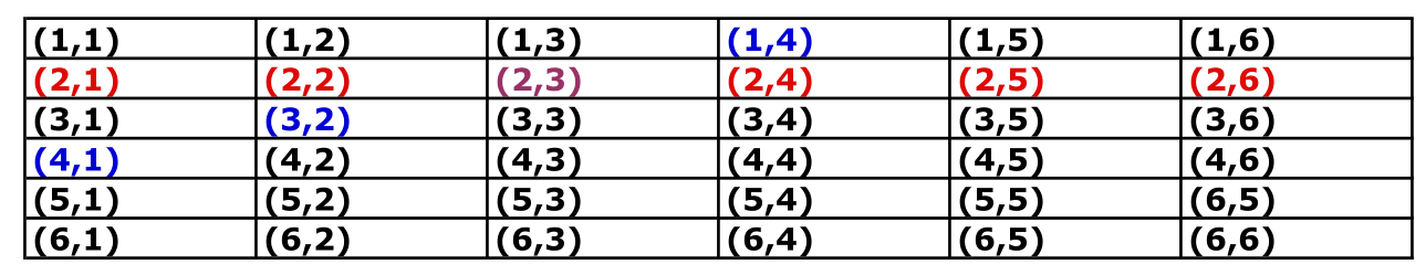
As we see in the table, the only scenario where we have \(A\) is when we obtain \(3\) in the second throw. Since the event “obtaining a 3” for one of the dice, has a probability\(=1/6\):
\(\text{Pr}\{\text{getting 5 given 2 in the first throw}\}= \text{Pr}\{\text{getting 3 in the second throw}\}=1/6.\)
Also, sometimes the probability can change drastically. For example, suppose that in our example we have 6 in the first throw. Then, the probability of observing 5 in two draws is zero(!)
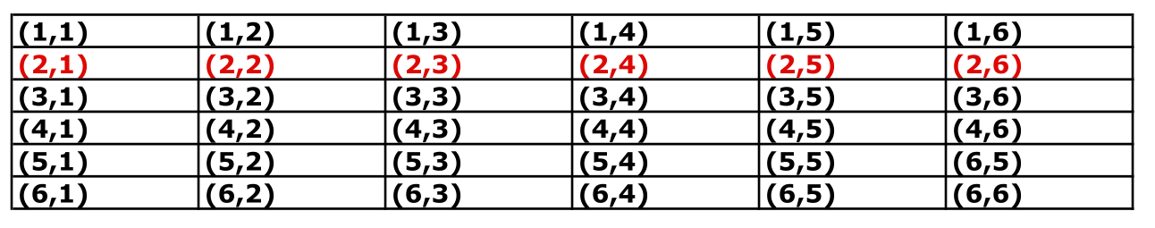
Let us come back to the example of the two dice and assess whether the formula applies. Let us define the event \(B\) as “obtaining a 2 on the first throw”, i.e.
The probability of this event can be computed as follows:
\[\begin{eqnarray} P(B) &=& Pr\left\{ (2,1) \cup (2,2) \cup (2,3) \cup (2,4) \cup (2,5) \cup (2,6) \right\} \\ &=& Pr(2,1) + Pr(2,2) + Pr(2,3) + Pr(2,4) + Pr(2,5) + Pr(2,6) \\ &=& 6/36 =1/6 \end{eqnarray}\]
Let us now focus on the event \(A \cap B\), i.e. “sum of both dice = 5” and “getting a 2 on the first throw**. As we have seen in the previous tables, this event arises only when the second die yields a 3, i.e.
Hence, \(P(A \cap B) = Pr (2,3) = 1/36\) and thus: \[ P(A\vert B) = \frac{P(A \cap B)}{P(B)} = \frac{1/36}{1/6} = \frac{1}{6}. \]
3.5 Independence
Clearly, if \(P(A\vert B) \neq P(A)\), then \(A\) and \(B\) are .
3.5.1 Another characterisation
Two events \(A\) and \(B\) are independent if \[P(A \vert B) = {P(A)},\] now by definition of conditional probability we know that \[P(A \vert B) = \frac{P(A \cap B)}{P(B)},\] so we have \[P(A) = \frac{P(A \cap B)}{P(B)},\] and rearranging the terms, we find that two events are independent iif \[P(A\cap B) = P(A) P(B).\]