Chapter 13 Basic Statistics
Lander's chapter 14 Basic Statistics
#t test, ANOVA
x <- sample(x=4, size = 10, replace = T)
x
## [1] 1 4 3 1 4 3 1 4 3 2x <- sample(x=1:200, size = 100, replace = T)
x## [1] 107 77 37 123 161 135 14 4 91 198 1 136 1 188 32 122 86 8 13 198 128 172
## [23] 39 194 168 19 65 83 13 115 98 105 37 194 52 5 150 134 24 150 148 56 29 129
## [45] 43 159 92 170 178 132 146 165 166 104 137 161 57 178 8 32 155 50 46 139 93 183
## [67] 83 99 65 76 164 99 160 40 185 98 166 37 66 107 9 185 87 142 110 14 43 30
## [89] 107 51 60 15 78 69 31 64 57 83 150 3x <- sample(x=1:100, size = 100, replace = T)
mean(x)## [1] 50.33y<- x
y[sample(x=1:100, size = 20, replace = F)]<- NA
y## [1] 1 51 100 22 NA 15 NA NA 12 18 94 26 55 NA 51 66 59 55 NA 44 95 10
## [23] NA 16 12 100 71 22 20 NA 7 58 NA 80 79 25 58 NA 22 33 39 1 12 26
## [45] 97 NA 54 77 36 97 88 62 52 NA 84 80 NA NA 100 92 NA NA 98 21 25 27
## [67] 45 56 33 38 18 32 24 34 62 34 98 1 44 NA 74 88 95 64 99 87 7 NA
## [89] NA 4 57 14 3 90 NA 10 72 69 NA 82mean(y)## [1] NAmean(y, na.rm = T)## [1] 49.7375grades <- c(95, 72, 87, 66)
weights <- c(1/2, 1/4, 1/8, 1/8)
tem <- grades*weights
tem## [1] 47.500 18.000 10.875 8.250sum(tem)## [1] 84.625weighted.mean(x=grades, w=weights)## [1] 84.625mean(x)## [1] 50.33var(x)## [1] 977.1526sum((x-mean(x))^2)/(length(x)-1)## [1] 977.1526sd(x)## [1] 31.25944sqrt(var(x))## [1] 31.25944#sd(y)
sd(y, na.rm = T)## [1] 31.66308min(x)## [1] 1max(x)## [1] 100median(x)## [1] 53.5#median(y)
median(y, na.rm = T)## [1] 51summary(y)## Min. 1st Qu. Median Mean 3rd Qu. Max. NA's
## 1.00 22.00 51.00 49.74 79.25 100.00 20quantile(x, probs = c(0.25, 0.75))## 25% 75%
## 23.5 79.0quantile(x)[c(2,4)]## 25% 75%
## 23.5 79.0#quantile(y, probs = c(0.25, 0.75))
quantile(y, probs = c(0.25, 0.75), na.rm = T)## 25% 75%
## 22.00 79.25quantile(x, probs = c(0.1, 0.25, 0.5, 0.75, 0.99))## 10% 25% 50% 75% 99%
## 9.7 23.5 53.5 79.0 100.0require(ggplot2)
head(economics)## # A tibble: 6 x 6
## date pce pop psavert uempmed unemploy
## <date> <dbl> <dbl> <dbl> <dbl> <dbl>
## 1 1967-07-01 507. 198712 12.6 4.5 2944
## 2 1967-08-01 510. 198911 12.6 4.7 2945
## 3 1967-09-01 516. 199113 11.9 4.6 2958
## 4 1967-10-01 512. 199311 12.9 4.9 3143
## 5 1967-11-01 517. 199498 12.8 4.7 3066
## 6 1967-12-01 525. 199657 11.8 4.8 3018cor(economics$pce, economics$psavert)## [1] -0.7928546#cor(economics$psavert, economics$pce)
xPart <- economics$pce-mean(economics$pce)
yPart <- economics$psavert-mean(economics$psavert)
nMinusOne <- nrow(economics)-1
xSD <- sd(economics$pce)
ySD <- sd(economics$psavert)
sum(xPart * yPart)/(nMinusOne * xSD * ySD)## [1] -0.7928546cor(economics[, c(2, 4:6)])## pce psavert uempmed unemploy
## pce 1.0000000 -0.7928546 0.7269616 0.6145176
## psavert -0.7928546 1.0000000 -0.3251377 -0.3093769
## uempmed 0.7269616 -0.3251377 1.0000000 0.8693097
## unemploy 0.6145176 -0.3093769 0.8693097 1.0000000GGally::ggpairs(economics[, c(2, 4:6)])## plot: [1,1] [===>--------------------------------------------------------------] 6% est: 0s
## plot: [1,2] [=======>----------------------------------------------------------] 12% est: 0s
## plot: [1,3] [===========>------------------------------------------------------] 19% est: 0s
## plot: [1,4] [===============>--------------------------------------------------] 25% est: 0s
## plot: [2,1] [====================>---------------------------------------------] 31% est: 0s
## plot: [2,2] [========================>-----------------------------------------] 38% est: 0s
## plot: [2,3] [============================>-------------------------------------] 44% est: 0s
## plot: [2,4] [================================>---------------------------------] 50% est: 0s
## plot: [3,1] [====================================>-----------------------------] 56% est: 0s
## plot: [3,2] [========================================>-------------------------] 62% est: 0s
## plot: [3,3] [============================================>---------------------] 69% est: 0s
## plot: [3,4] [=================================================>----------------] 75% est: 0s
## plot: [4,1] [=====================================================>------------] 81% est: 0s
## plot: [4,2] [=========================================================>--------] 88% est: 0s
## plot: [4,3] [=============================================================>----] 94% est: 0s
## plot: [4,4] [==================================================================]100% est: 0s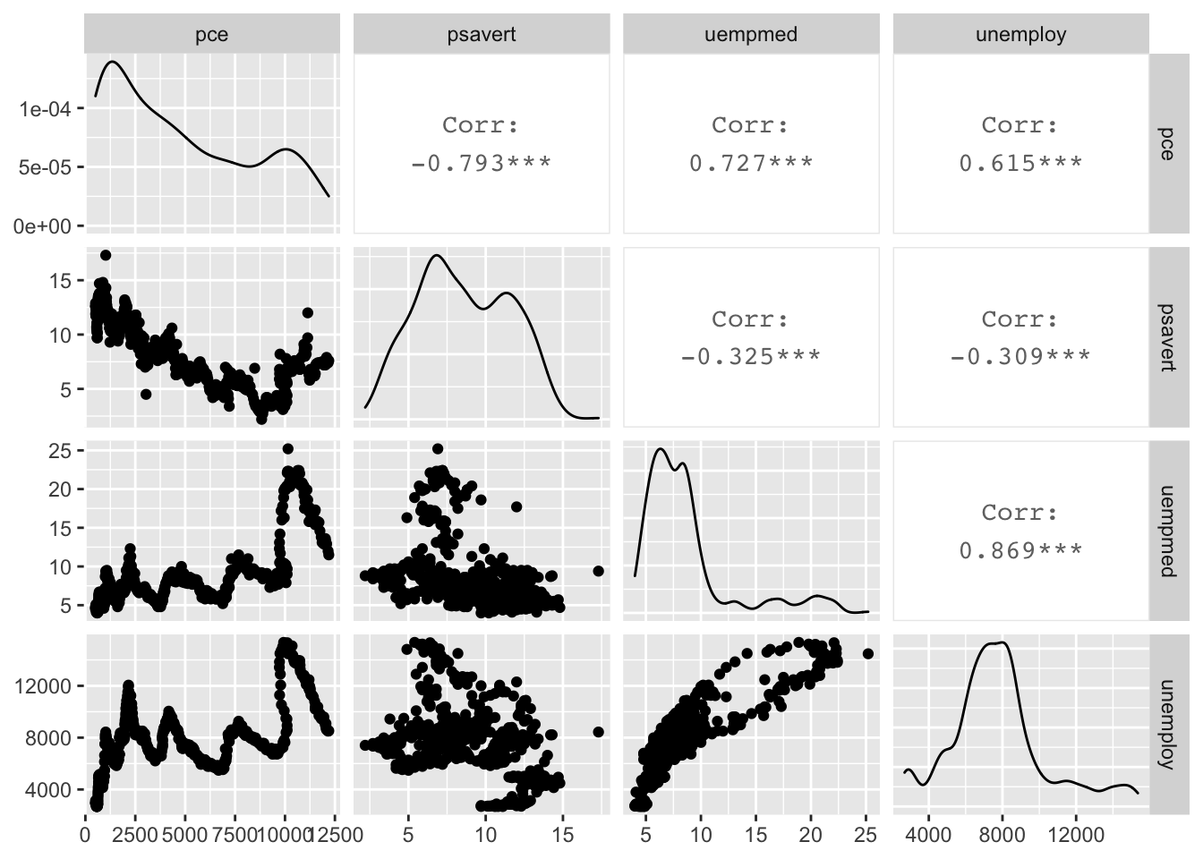
?ggpairs

rm(list = ls())
require(reshape2)
require(scales)
econCor <- cor(economics[, c(2, 4:6)])
econCor
## pce psavert uempmed unemploy
## pce 1.0000000 -0.7928546 0.7269616 0.6145176
## psavert -0.7928546 1.0000000 -0.3251377 -0.3093769
## uempmed 0.7269616 -0.3251377 1.0000000 0.8693097
## unemploy 0.6145176 -0.3093769 0.8693097 1.0000000#note the difference between the uses of variable.name and varnames
#id.vars does not give column names
ecomMelt <- melt(econCor, varnames=c("x", "y"), value.name = "Correlation")
ecomMelt <- melt(econCor, id.vars=c("x", "y"), value.name = "Correlation")
names(ecomMelt)## [1] "Var1" "Var2" "Correlation"#Decreasing=F by default
ecomMelt <- ecomMelt[order(ecomMelt$Correlation),]
ecomMelt## Var1 Var2 Correlation
## 2 psavert pce -0.7928546
## 5 pce psavert -0.7928546
## 7 uempmed psavert -0.3251377
## 10 psavert uempmed -0.3251377
## 8 unemploy psavert -0.3093769
## 14 psavert unemploy -0.3093769
## 4 unemploy pce 0.6145176
## 13 pce unemploy 0.6145176
## 3 uempmed pce 0.7269616
## 9 pce uempmed 0.7269616
## 12 unemploy uempmed 0.8693097
## 15 uempmed unemploy 0.8693097
## 1 pce pce 1.0000000
## 6 psavert psavert 1.0000000
## 11 uempmed uempmed 1.0000000
## 16 unemploy unemploy 1.0000000m <- c(9,9,NA,3,NA,5,8,1,10,4)
n <- c(2,NA,1,6,6,4, 1,1,6,7)
p <- c(8,4,3,9,10,NA,3,NA,9,9)
q <- c(10,10,7,8,4,2,8,5,5,2)
r <- c(1,9,7,6,5,6,2,7,9,10)
theMat <- cbind(m,n,p,q,r)
dim(theMat)## [1] 10 5cor(theMat, use = "everything") #entirety of all columns must be free of NAs## m n p q r
## m 1 NA NA NA NA
## n NA 1 NA NA NA
## p NA NA 1 NA NA
## q NA NA NA 1.0000000 -0.4242958
## r NA NA NA -0.4242958 1.0000000#cor(theMat, use = "all.obs")
cor(theMat, use = "complete.obs")## m n p q r
## m 1.0000000 -0.5228840 -0.2893527 0.2974398 -0.3459470
## n -0.5228840 1.0000000 0.8090195 -0.7448453 0.9350718
## p -0.2893527 0.8090195 1.0000000 -0.3613720 0.6221470
## q 0.2974398 -0.7448453 -0.3613720 1.0000000 -0.9059384
## r -0.3459470 0.9350718 0.6221470 -0.9059384 1.0000000#keep only rows where every entry is not NA
cor(theMat, use = "complete.obs")## m n p q r
## m 1.0000000 -0.5228840 -0.2893527 0.2974398 -0.3459470
## n -0.5228840 1.0000000 0.8090195 -0.7448453 0.9350718
## p -0.2893527 0.8090195 1.0000000 -0.3613720 0.6221470
## q 0.2974398 -0.7448453 -0.3613720 1.0000000 -0.9059384
## r -0.3459470 0.9350718 0.6221470 -0.9059384 1.0000000cor(theMat, use = "na.or.complete")## m n p q r
## m 1.0000000 -0.5228840 -0.2893527 0.2974398 -0.3459470
## n -0.5228840 1.0000000 0.8090195 -0.7448453 0.9350718
## p -0.2893527 0.8090195 1.0000000 -0.3613720 0.6221470
## q 0.2974398 -0.7448453 -0.3613720 1.0000000 -0.9059384
## r -0.3459470 0.9350718 0.6221470 -0.9059384 1.0000000cor(theMat[c(1,4,7,9,10),])## m n p q r
## m 1.0000000 -0.5228840 -0.2893527 0.2974398 -0.3459470
## n -0.5228840 1.0000000 0.8090195 -0.7448453 0.9350718
## p -0.2893527 0.8090195 1.0000000 -0.3613720 0.6221470
## q 0.2974398 -0.7448453 -0.3613720 1.0000000 -0.9059384
## r -0.3459470 0.9350718 0.6221470 -0.9059384 1.0000000identical(cor(theMat, use = "complete.obs"), cor(theMat[c(1,4,7,9,10),]))## [1] TRUEcor(theMat, use = "complete.obs")## m n p q r
## m 1.0000000 -0.5228840 -0.2893527 0.2974398 -0.3459470
## n -0.5228840 1.0000000 0.8090195 -0.7448453 0.9350718
## p -0.2893527 0.8090195 1.0000000 -0.3613720 0.6221470
## q 0.2974398 -0.7448453 -0.3613720 1.0000000 -0.9059384
## r -0.3459470 0.9350718 0.6221470 -0.9059384 1.0000000cor(theMat[,c("m","n")], use = "complete.obs")## m n
## m 1.00000000 -0.02511812
## n -0.02511812 1.00000000data(tips, package = "reshape2")
head(tips)## total_bill tip sex smoker day time size
## 1 16.99 1.01 Female No Sun Dinner 2
## 2 10.34 1.66 Male No Sun Dinner 3
## 3 21.01 3.50 Male No Sun Dinner 3
## 4 23.68 3.31 Male No Sun Dinner 2
## 5 24.59 3.61 Female No Sun Dinner 4
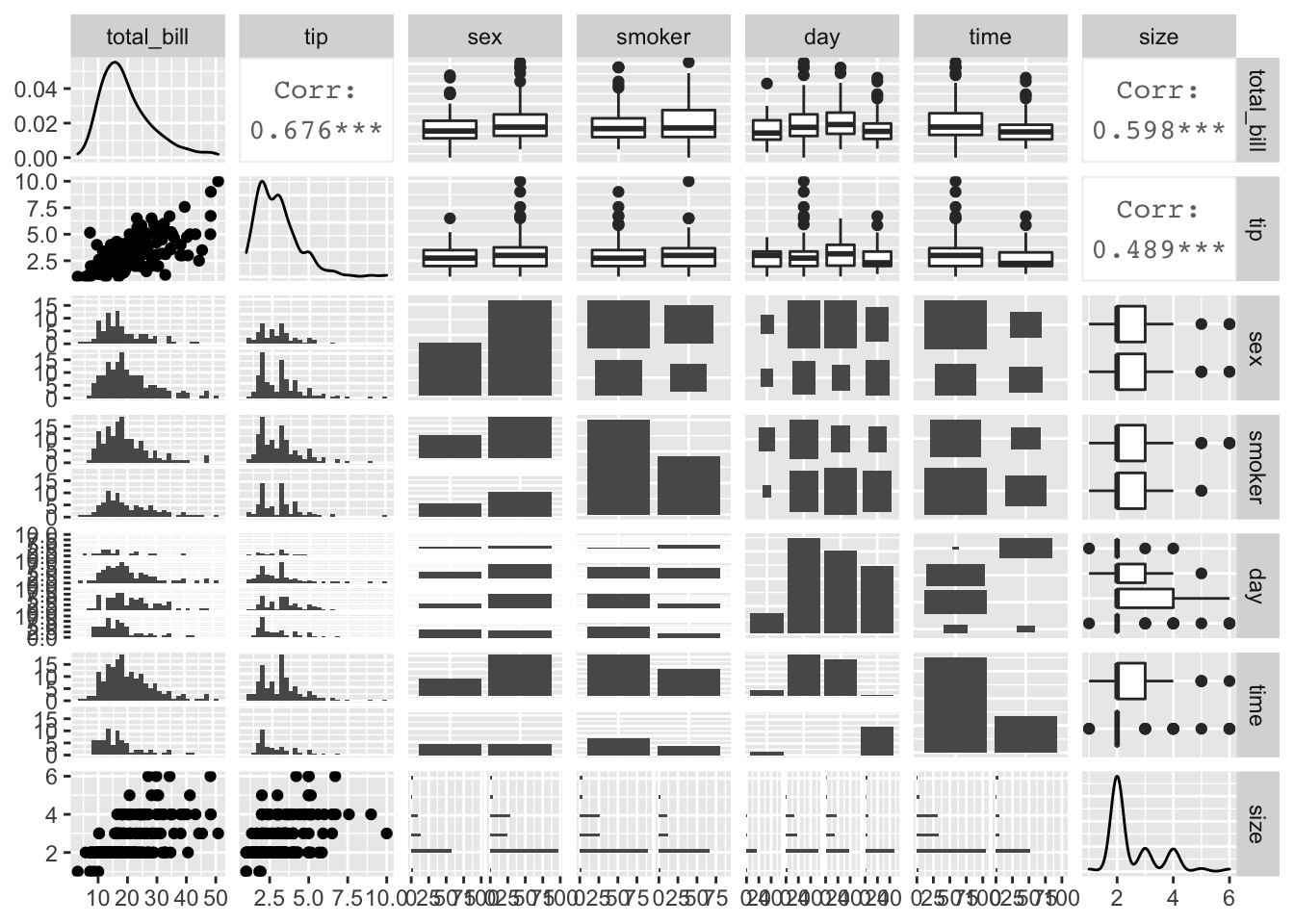
## 6 25.29 4.71 Male No Sun Dinner 4GGally::ggpairs(tips)##
plot: [1,1] [>-----------------------------------------------------------------] 2% est: 0s
plot: [1,2] [==>---------------------------------------------------------------] 4% est: 1s
plot: [1,3] [===>--------------------------------------------------------------] 6% est: 2s
plot: [1,4] [====>-------------------------------------------------------------] 8% est: 2s
plot: [1,5] [======>-----------------------------------------------------------] 10% est: 2s
plot: [1,6] [=======>----------------------------------------------------------] 12% est: 2s
plot: [1,7] [========>---------------------------------------------------------] 14% est: 2s
plot: [2,1] [==========>-------------------------------------------------------] 16% est: 2s
plot: [2,2] [===========>------------------------------------------------------] 18% est: 2s
plot: [2,3] [============>-----------------------------------------------------] 20% est: 2s
plot: [2,4] [==============>---------------------------------------------------] 22% est: 2s
plot: [2,5] [===============>--------------------------------------------------] 24% est: 2s
plot: [2,6] [=================>------------------------------------------------] 27% est: 2s
plot: [2,7] [==================>-----------------------------------------------] 29% est: 2s
plot: [3,1] [===================>----------------------------------------------] 31% est: 2s `stat_bin()` using `bins = 30`. Pick better value with `binwidth`.
##
plot: [3,2] [=====================>--------------------------------------------] 33% est: 2s `stat_bin()` using `bins = 30`. Pick better value with `binwidth`.
##
plot: [3,3] [======================>-------------------------------------------] 35% est: 2s
plot: [3,4] [=======================>------------------------------------------] 37% est: 2s
plot: [3,5] [=========================>----------------------------------------] 39% est: 2s
plot: [3,6] [==========================>---------------------------------------] 41% est: 2s
plot: [3,7] [===========================>--------------------------------------] 43% est: 2s
plot: [4,1] [=============================>------------------------------------] 45% est: 2s `stat_bin()` using `bins = 30`. Pick better value with `binwidth`.
##
plot: [4,2] [==============================>-----------------------------------] 47% est: 2s `stat_bin()` using `bins = 30`. Pick better value with `binwidth`.
##
plot: [4,3] [===============================>----------------------------------] 49% est: 2s
plot: [4,4] [=================================>--------------------------------] 51% est: 2s
plot: [4,5] [==================================>-------------------------------] 53% est: 2s
plot: [4,6] [===================================>------------------------------] 55% est: 2s
plot: [4,7] [=====================================>----------------------------] 57% est: 1s
plot: [5,1] [======================================>---------------------------] 59% est: 1s `stat_bin()` using `bins = 30`. Pick better value with `binwidth`.
##
plot: [5,2] [=======================================>--------------------------] 61% est: 1s `stat_bin()` using `bins = 30`. Pick better value with `binwidth`.
##
plot: [5,3] [=========================================>------------------------] 63% est: 1s
plot: [5,4] [==========================================>-----------------------] 65% est: 1s
plot: [5,5] [===========================================>----------------------] 67% est: 1s
plot: [5,6] [=============================================>--------------------] 69% est: 1s
plot: [5,7] [==============================================>-------------------] 71% est: 1s
plot: [6,1] [===============================================>------------------] 73% est: 1s `stat_bin()` using `bins = 30`. Pick better value with `binwidth`.
##
plot: [6,2] [=================================================>----------------] 76% est: 1s `stat_bin()` using `bins = 30`. Pick better value with `binwidth`.
##
plot: [6,3] [==================================================>---------------] 78% est: 1s
plot: [6,4] [====================================================>-------------] 80% est: 1s
plot: [6,5] [=====================================================>------------] 82% est: 1s
plot: [6,6] [======================================================>-----------] 84% est: 1s
plot: [6,7] [========================================================>---------] 86% est: 1s
plot: [7,1] [=========================================================>--------] 88% est: 1s
plot: [7,2] [==========================================================>-------] 90% est: 0s
plot: [7,3] [============================================================>-----] 92% est: 0s `stat_bin()` using `bins = 30`. Pick better value with `binwidth`.
##
plot: [7,4] [=============================================================>----] 94% est: 0s `stat_bin()` using `bins = 30`. Pick better value with `binwidth`.
##
plot: [7,5] [==============================================================>---] 96% est: 0s `stat_bin()` using `bins = 30`. Pick better value with `binwidth`.
##
plot: [7,6] [================================================================>-] 98% est: 0s `stat_bin()` using `bins = 30`. Pick better value with `binwidth`.
##
plot: [7,7] [==================================================================]100% est: 0s
#covariance
cov(economics$pce, economics$psavert)
## [1] -8359.069cov(economics[, c(2, 4:6)])## pce psavert uempmed unemploy
## pce 12650851.944 -8359.069071 10618.386190 5774578.978
## psavert -8359.069 8.786360 -3.957847 -2422.805
## uempmed 10618.386 -3.957847 16.864531 9431.652
## unemploy 5774578.978 -2422.805358 9431.652268 6979948.309identical(cov(economics$pce, economics$psavert),
cor(economics$pce, economics$psavert)*
sd(economics$pce)*sd(economics$psavert))## [1] TRUEhead(tips)## total_bill tip sex smoker day time size
## 1 16.99 1.01 Female No Sun Dinner 2
## 2 10.34 1.66 Male No Sun Dinner 3
## 3 21.01 3.50 Male No Sun Dinner 3
## 4 23.68 3.31 Male No Sun Dinner 2
## 5 24.59 3.61 Female No Sun Dinner 4
## 6 25.29 4.71 Male No Sun Dinner 4unique(tips$sex)## [1] Female Male
## Levels: Female Maleunique(tips$day)## [1] Sun Sat Thur Fri
## Levels: Fri Sat Sun Thur#h0: the average tip is equal to 2.5
mean(tips$tip)## [1] 2.998279#leave question
t.test(tips$tip, alternative = "two.sided", mu = 2.5)##
## One Sample t-test
##
## data: tips$tip
## t = 5.6253, df = 243, p-value = 5.08e-08
## alternative hypothesis: true mean is not equal to 2.5
## 95 percent confidence interval:
## 2.823799 3.172758
## sample estimates:
## mean of x
## 2.998279dim(tips)## [1] 244 7z <- (mean(tips$tip)-2.5)/(sd(tips$tip)/sqrt(length(tips$tip)))
(1-pnorm(z, 0, 1))*2## [1] 1.851998e-08randT <- rt(30000, df=nrow(tips)-1)
NROW(tips)## [1] 244nrow(tips)## [1] 244tipTTest <- t.test(tips$tip, alternative = "two.sided", mu=2.5)
ggplot(data.frame(x=randT))+
geom_density(aes(x=x), fill="grey", color="grey")+
geom_vline(xintercept = tipTTest$statistic)+
geom_vline(xintercept = mean(randT)+c(-2,2)*sd(randT), linetype=2)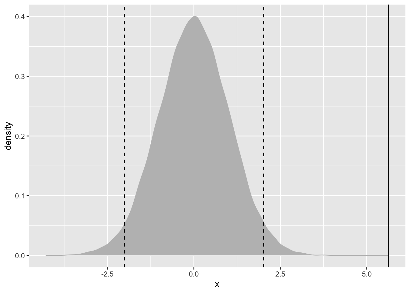
names(tipTTest)## [1] "statistic" "parameter" "p.value" "conf.int" "estimate" "null.value"
## [7] "stderr" "alternative" "method" "data.name"tipTTest$statistic## t
## 5.625287#H0: t is greater than 2.5
t.test(tips$tip, alternative="greater", mu=2.5)##
## One Sample t-test
##
## data: tips$tip
## t = 5.6253, df = 243, p-value = 2.54e-08
## alternative hypothesis: true mean is greater than 2.5
## 95 percent confidence interval:
## 2.852023 Inf
## sample estimates:
## mean of x
## 2.998279#two-sample t-text
#a traditional t-text requires same variance
#Welch two-sample t-test can handle differing variances
aggregate(tip ~ sex, data = tips, var)## sex tip
## 1 Female 1.344428
## 2 Male 2.217424#test for normality
shapiro.test(tips$tip)##
## Shapiro-Wilk normality test
##
## data: tips$tip
## W = 0.89781, p-value = 8.2e-12shapiro.test(tips$tip[tips$sex=="Male"])##
## Shapiro-Wilk normality test
##
## data: tips$tip[tips$sex == "Male"]
## W = 0.87587, p-value = 3.708e-10shapiro.test(tips$tip[tips$sex=="Female"])##
## Shapiro-Wilk normality test
##
## data: tips$tip[tips$sex == "Female"]
## W = 0.95678, p-value = 0.005448hist(tips$tip)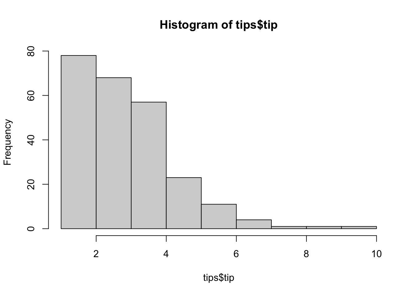
#all the tests fail so inspect visually
#H0: normality

ggplot(tips, aes(x=tip, fill=sex))+
  geom_histogram(binwidth=0.5, alpha=0.5) #alpha: transparency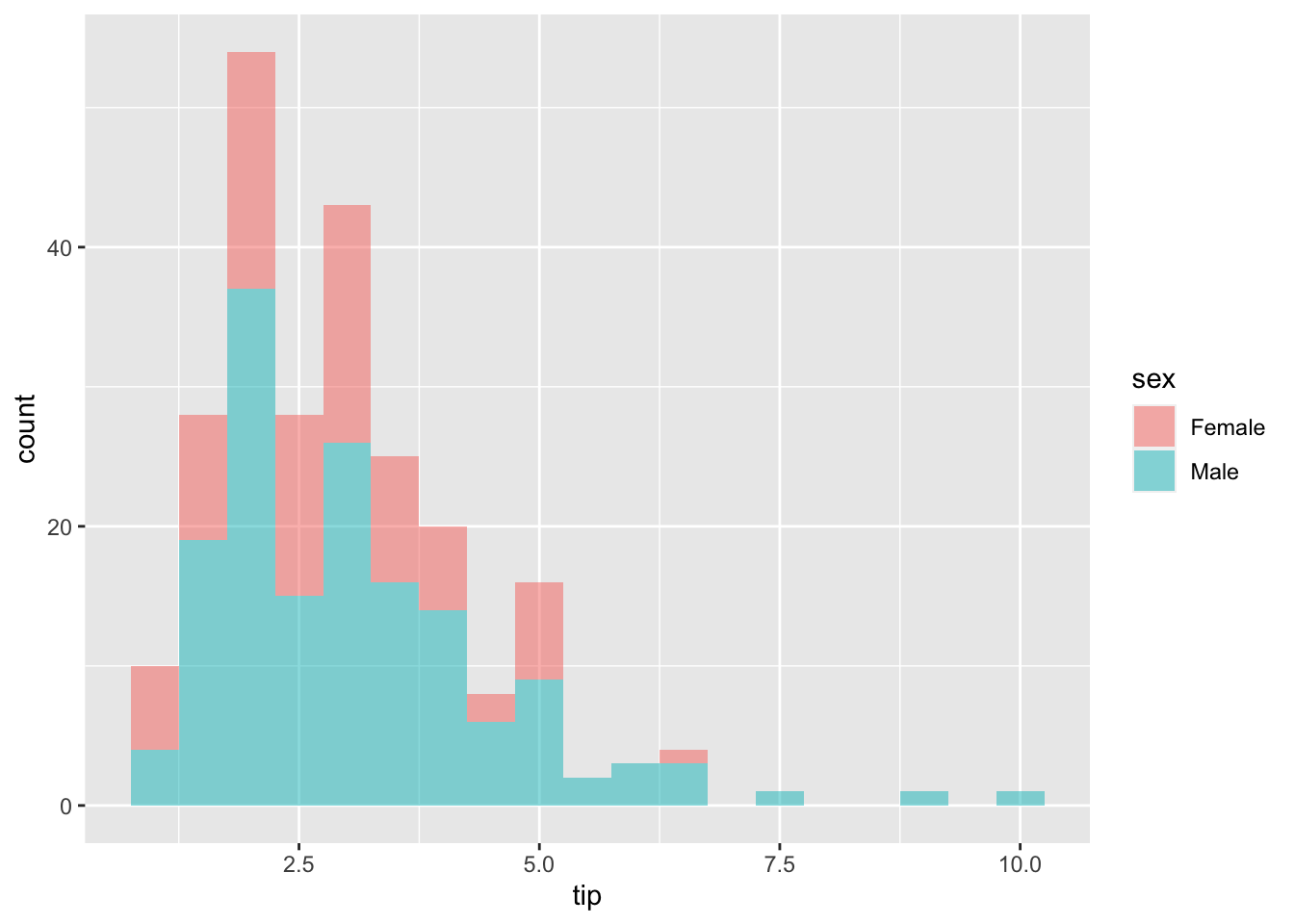
#neither the standard F-test (var.text) nor Bartlett test (bartlett.text) will suffice

#nonparametric Ansari-Bradley to examine equality of variances
ansari.test(tip~sex, tips)
##
## Ansari-Bradley test
##
## data: tip by sex
## AB = 5582.5, p-value = 0.376
## alternative hypothesis: true ratio of scales is not equal to 1#variances are equal
#so can apply standard two-sample t-test
t.test(tip~sex, data = tips, var.equal=T)##
## Two Sample t-test
##
## data: tip by sex
## t = -1.3879, df = 242, p-value = 0.1665
## alternative hypothesis: true difference in means is not equal to 0
## 95 percent confidence interval:
## -0.6197558 0.1074167
## sample estimates:
## mean in group Female mean in group Male
## 2.833448 3.089618#female and male are tipped roughly equally
#var.equal=FALSE (the default) would run the Welch test
names(tips)## [1] "total_bill" "tip" "sex" "smoker" "day" "time" "size"require(plyr)
tipSummary <-
ddply(tips, "sex", summarize,
tip.mean=mean(tip), tip.sd=sd(tip),
Lower=tip.mean-2*tip.sd/sqrt(NROW(tip)),
Upper=tip.mean+2*tip.sd/sqrt(NROW(tip)))
str(tips)## 'data.frame': 244 obs. of 7 variables:
## $ total_bill: num 17 10.3 21 23.7 24.6 ...
## $ tip : num 1.01 1.66 3.5 3.31 3.61 4.71 2 3.12 1.96 3.23 ...
## $ sex : Factor w/ 2 levels "Female","Male": 1 2 2 2 1 2 2 2 2 2 ...
## $ smoker : Factor w/ 2 levels "No","Yes": 1 1 1 1 1 1 1 1 1 1 ...
## $ day : Factor w/ 4 levels "Fri","Sat","Sun",..: 3 3 3 3 3 3 3 3 3 3 ...
## $ time : Factor w/ 2 levels "Dinner","Lunch": 1 1 1 1 1 1 1 1 1 1 ...
## $ size : int 2 3 3 2 4 4 2 4 2 2 ...nrow(tips)## [1] 244nrow(tips$tip)## NULLNROW(tips$tip)#TREAT a vector as 1-column matrix## [1] 244?NROW
ggplot(tipSummary, aes(x=tip.mean, y=sex))+
geom_point()+
geom_errorbarh(aes(xmin=Lower, xmax=Upper),
height=.2)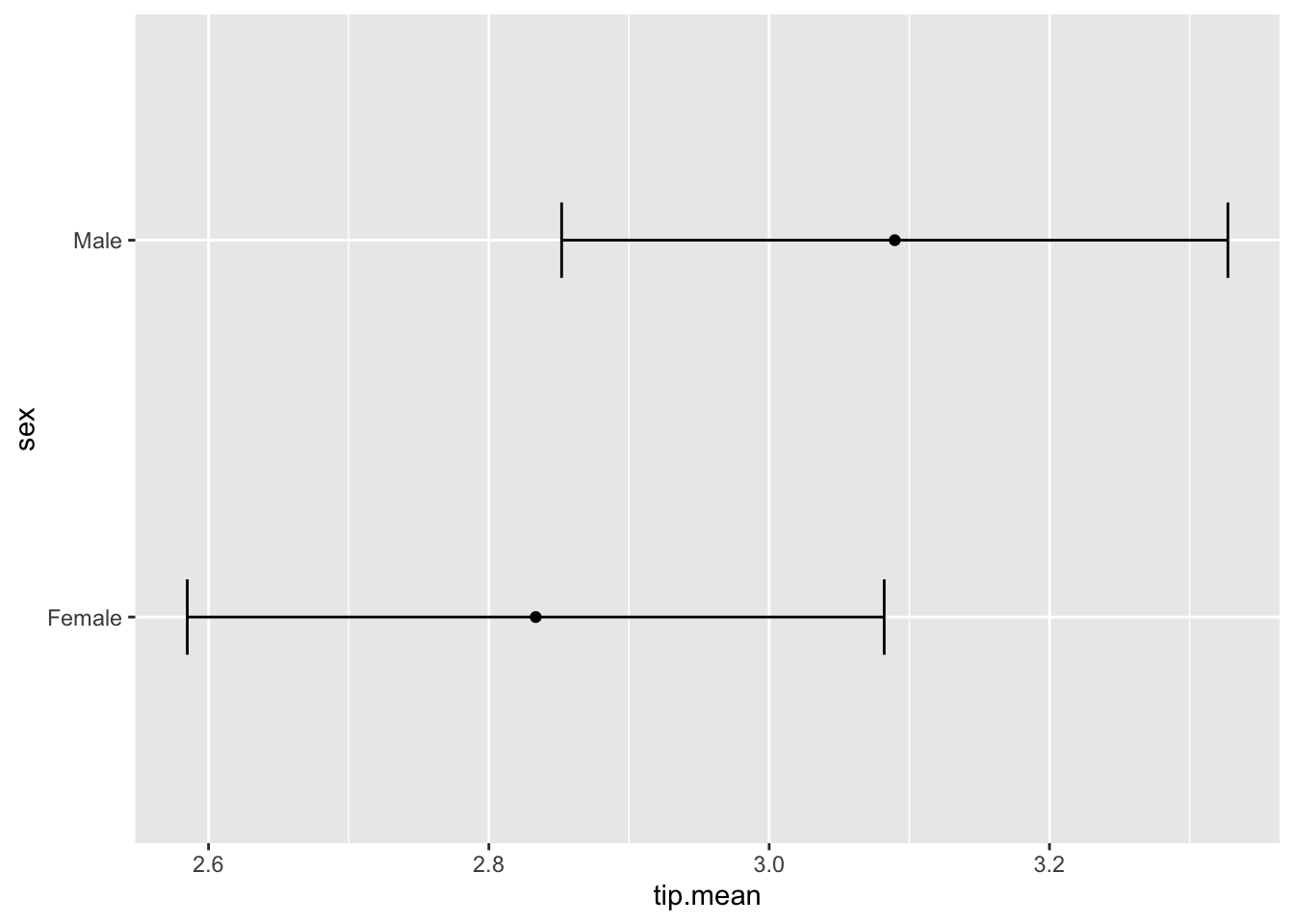
names(tipSummary)## [1] "sex" "tip.mean" "tip.sd" "Lower" "Upper"#geom_errorbar vs. geom_errorbarh: be careful with x,y limits
#paired two-sample t-test: observations in pairs are correlated
#vs. independent two-sample t-test