Chapter 12 Probability Distributions
Lander's chapter 14 Probability Distributions
#####################################
#chapter14 probability distributions#
#####################################
library(tidyverse)
library(reshape2)
#normal distribution
rnorm(n=10)
## [1] 0.10742845 1.47572316 0.87780092 1.06053657 0.73220495 3.55942400 0.16369035 0.08238296
## [9] 0.02358518 0.53158209rnorm(n=10, mean = 100, sd=20)## [1] 92.02657 126.03525 117.80587 92.62149 109.18156 88.88660 105.99909 114.34756 61.99287
## [10] 65.69723randNorm10 <- rnorm(10)
randNorm10## [1] 0.8488954 -0.4783605 -1.5271801 0.2886871 -1.7713282 1.5400277 0.5953859 -0.3749823
## [9] -1.6476411 -0.4338485dnorm(randNorm10)## [1] 0.27824584 0.35581194 0.12429742 0.38265990 0.08309753 0.12187234 0.33414485 0.37185756
## [9] 0.10266345 0.36310951#pdf of -1; mean=0, sd=1
#mathematically impossible
dnorm(-1, 0, 1)## [1] 0.2419707dnorm(c(-1, 0, 1))## [1] 0.2419707 0.3989423 0.2419707randNorm <- rnorm(30000)
randDensity <- dnorm(randNorm)
require(ggplot2)
ggplot(data.frame(x=randNorm, y=randDensity))+
aes(x=x, y=y)+
geom_point()+
labs(x="Random Normal Variables", y="Density")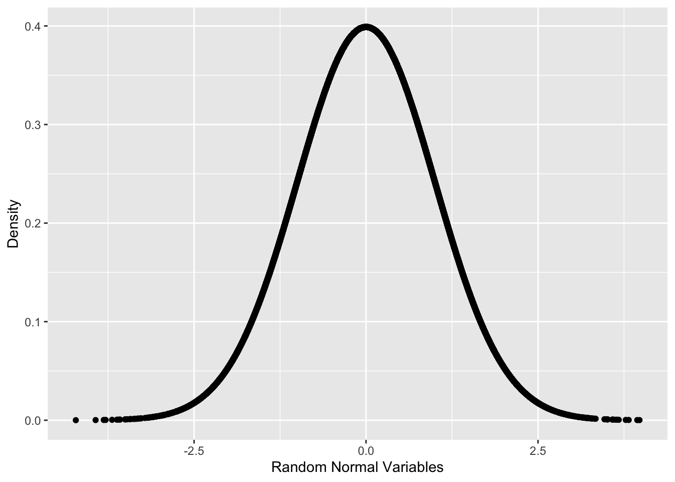
max(randNorm)## [1] 3.974804dnorm(4.5)## [1] 1.598374e-051-pnorm(4.5)## [1] 3.397673e-06randNorm10## [1] 0.8488954 -0.4783605 -1.5271801 0.2886871 -1.7713282 1.5400277 0.5953859 -0.3749823
## [9] -1.6476411 -0.4338485pnorm(randNorm10)## [1] 0.80203026 0.31619681 0.06335812 0.61358960 0.03825307 0.93822320 0.72420722 0.35383681
## [9] 0.04971317 0.33219921pnorm## function (q, mean = 0, sd = 1, lower.tail = TRUE, log.p = FALSE)
## .Call(C_pnorm, q, mean, sd, lower.tail, log.p)
## <bytecode: 0x10f85fe90>
## <environment: namespace:stats>pnorm(c(-3,0,3))## [1] 0.001349898 0.500000000 0.998650102pnorm(-1)## [1] 0.1586553#left-tailed by default
pnorm(1)-pnorm(0)## [1] 0.3413447pnorm(0)-pnorm(-1)## [1] 0.3413447pnorm(1)-pnorm(-1)## [1] 0.6826895#plot pnorm(-1)
p <- ggplot(data.frame(x=randNorm, y=randDensity))+
aes(x=x, y=y)+
geom_line()+
labs(x="x", y="Density")
p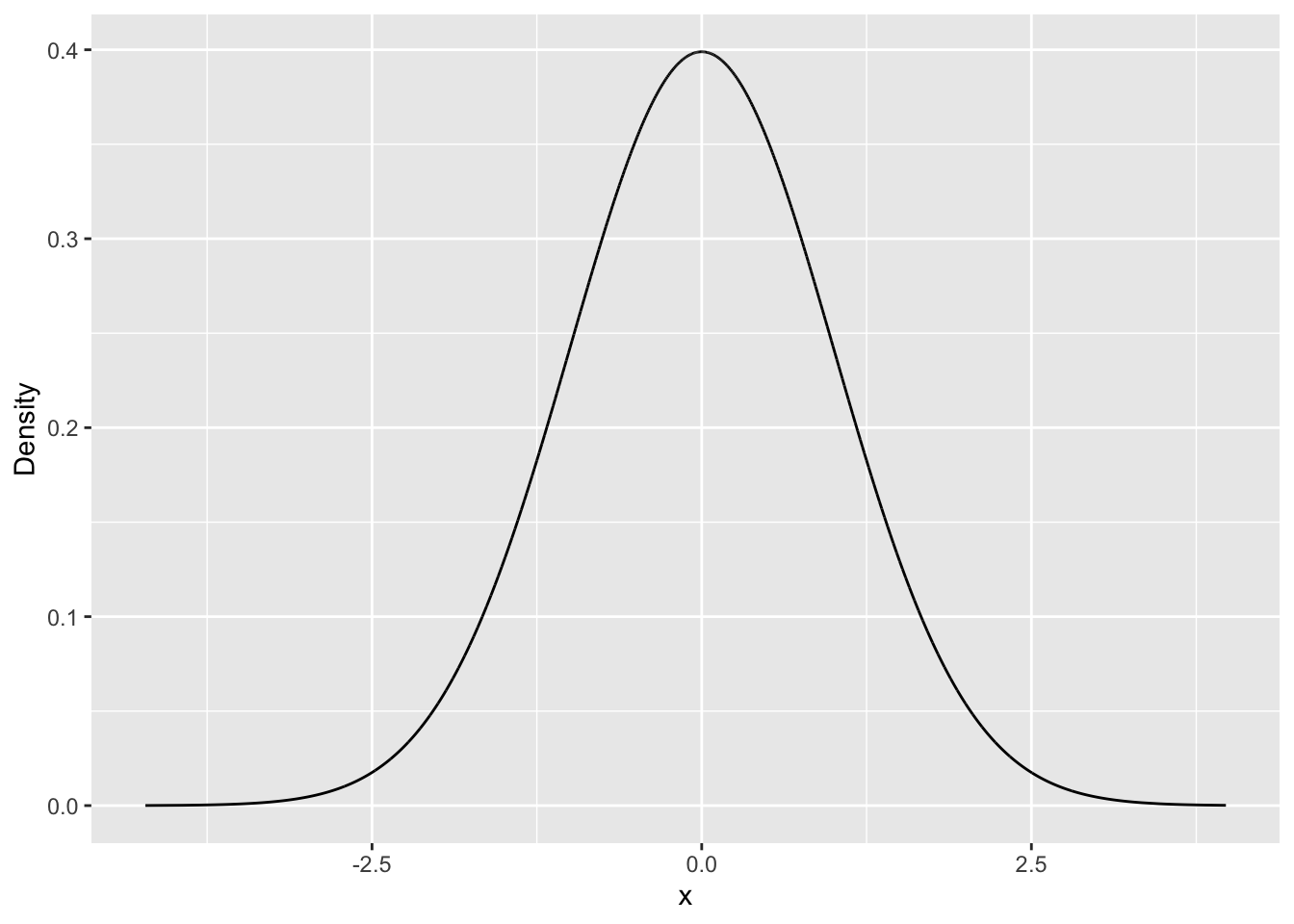
neg1Seq <- seq(from=min(randNorm), to=-1, by=0.1)
lessThanNeg1 <- data.frame(x=neg1Seq, y=dnorm(neg1Seq))
head(lessThanNeg1)
## x y
## 1 -4.218679 5.448609e-05
## 2 -4.118679 8.266641e-05
## 3 -4.018679 1.241737e-04
## 4 -3.918679 1.846661e-04
## 5 -3.818679 2.718953e-04
## 6 -3.718679 3.963450e-04lessThanNeg1 <- rbind(c(min(randNorm), 0),
lessThanNeg1,
c(max(lessThanNeg1$x),0))
p+geom_polygon(data = lessThanNeg1, aes(x=x,y=y))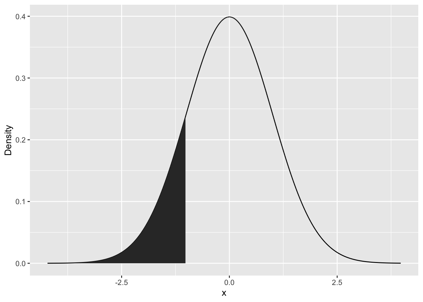
#plot pnorm(1)-pnorm(-1)
neg1Pos1Seq <- seq(from=-1, to=1, by=0.1)
neg1To1 <- data.frame(x=neg1Pos1Seq, y=dnorm(neg1Pos1Seq))
head(neg1To1)
## x y
## 1 -1.0 0.2419707
## 2 -0.9 0.2660852
## 3 -0.8 0.2896916
## 4 -0.7 0.3122539
## 5 -0.6 0.3332246
## 6 -0.5 0.3520653neg1To1 <- rbind(c(min(neg1To1$x),0),
neg1To1,
c(max(neg1To1$x),0))
#try the following codes:
#geom_polygon connects points in order:
#neg1To1 <- rbind(neg1To1,
# c(min(neg1To1$x),0),
# c(max(neg1To1$x),0))
p+geom_polygon(data=neg1To1, aes(x=x,y=y))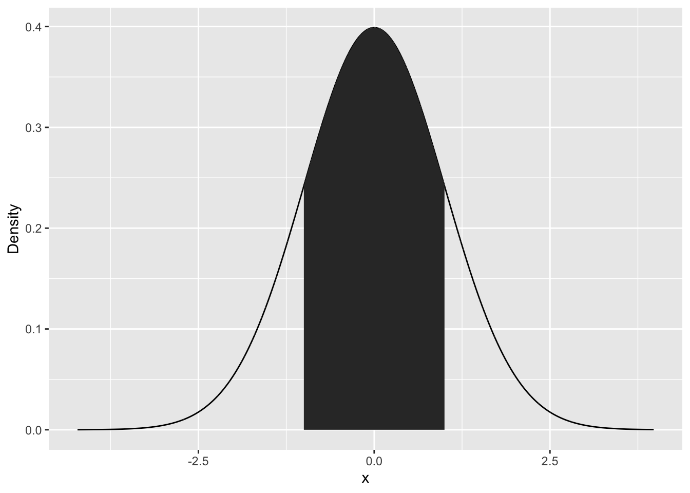
randProb <- pnorm(randNorm)
ggplot(data.frame(x=randNorm, y=randProb))+
  aes(x=x, y=y)+
  geom_point()+
  labs(x="Random Normal Variables", y="Probability")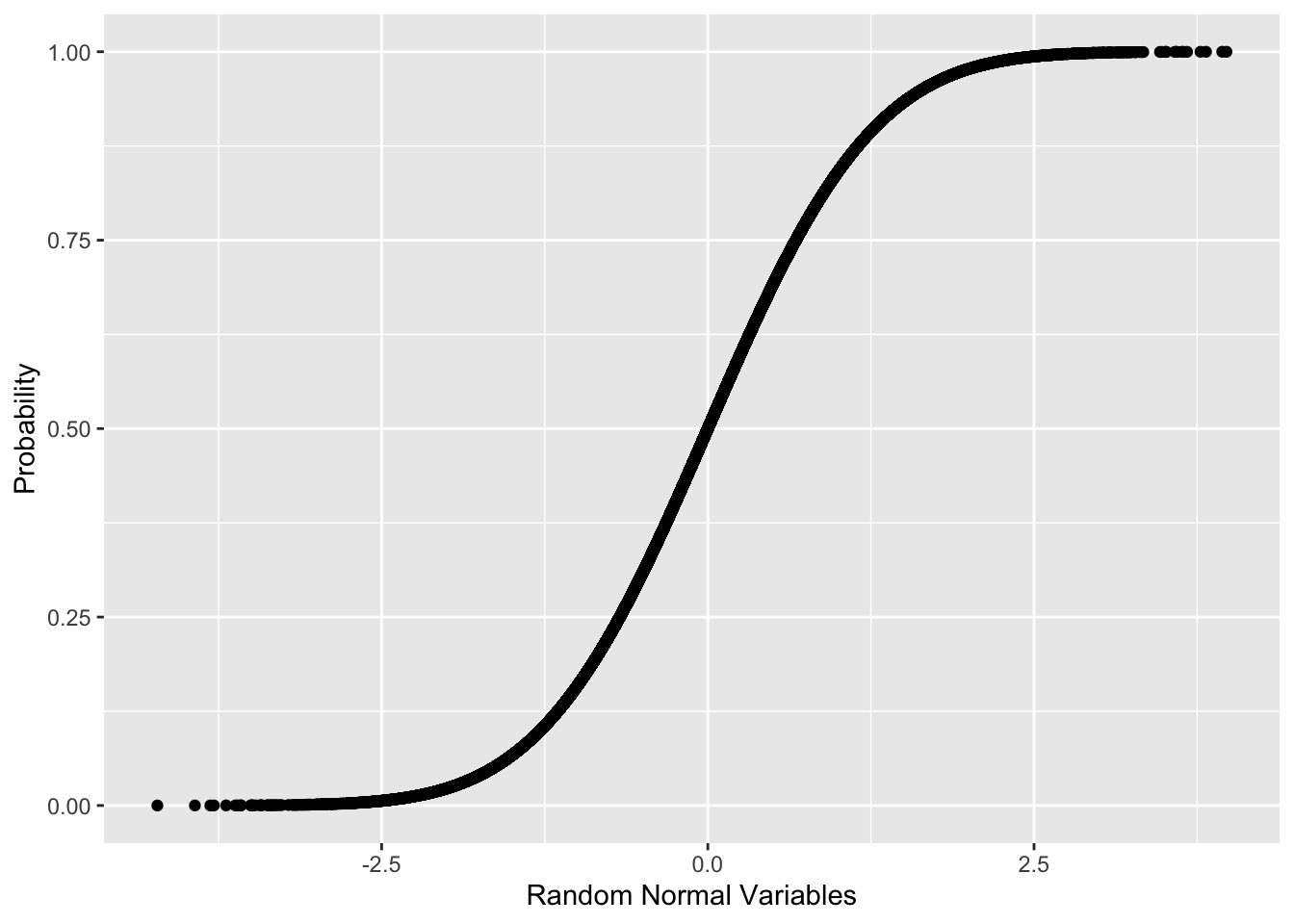
#note the position of aes()
ggplot(data.frame(x=randNorm, y=randProb), aes(x=x, y=y))+
  geom_point()+
  labs(x="Random Normal Variables", y="Probability")
qnorm(pnorm(randNorm10))## [1] 0.8488954 -0.4783605 -1.5271801 0.2886871 -1.7713282 1.5400277 0.5953859 -0.3749823
## [9] -1.6476411 -0.4338485all.equal(randNorm10, qnorm(pnorm(randNorm10)))## [1] TRUE#binomial distribution
rbinom(n=1, size = 10, prob = 0.4)## [1] 2?rbinom
#n>1, R generates the number of successes for each of the n sets of size trails
#n: number of observations/repeats; size: number of trials(sample size)
rbinom(5, 10, 0.4)## [1] 5 3 5 5 6rbinom(10, 10, 0.4)## [1] 1 4 5 5 5 6 3 2 5 5#Bernoulli
rbinom(n=1, size=1, prob = .4)## [1] 0rbinom(5, 1, .4)## [1] 0 0 0 0 0rbinom(10, 1, .4)## [1] 1 0 1 1 0 1 1 1 1 1#logit regression
#outcome = beta * indicator
#log(P(outcome=1)/1-P(outcome=1)) = beta*indicator
#exp(beta)/1+exp(beta)
binomData <- data.frame(Successes=rbinom(10000, 10, 0.3))
head(binomData)## Successes
## 1 5
## 2 0
## 3 0
## 4 4
## 5 6
## 6 3ggplot(binomData, aes(x=Successes))+
geom_histogram(binwidth = 1)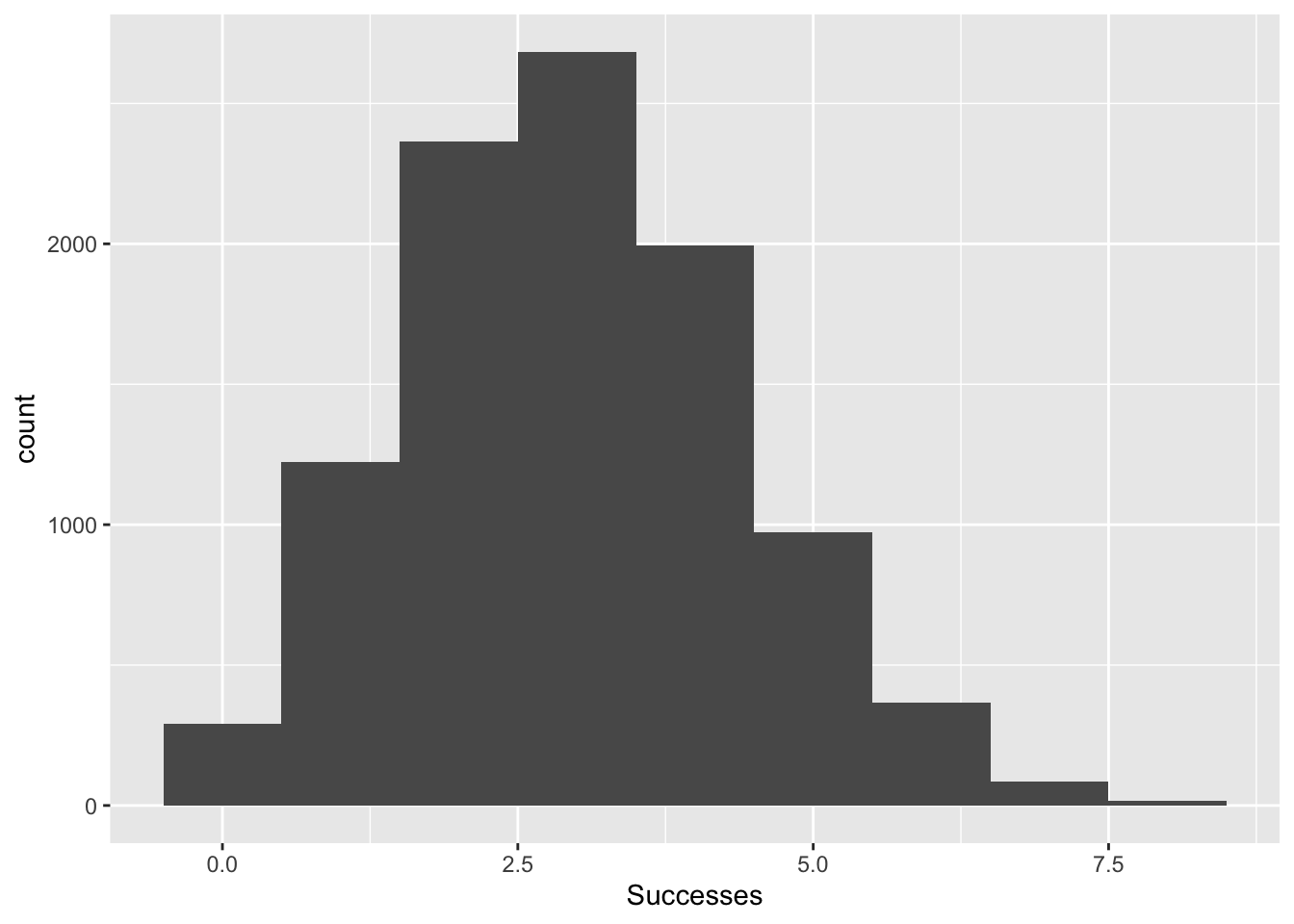
binom5 <- data.frame(Successes=rbinom(10000, 5, .3), size=5)
dim(binom5)
## [1] 10000 2head(binom5)## Successes size
## 1 2 5
## 2 3 5
## 3 3 5
## 4 2 5
## 5 1 5
## 6 2 5binom10 <- data.frame(Successes=rbinom(10000, 10, .3), size=10)
head(binom10)## Successes size
## 1 1 10
## 2 4 10
## 3 3 10
## 4 3 10
## 5 1 10
## 6 6 10binom100 <- data.frame(Successes=rbinom(10000, size = 100, prob = 0.3), size=100)
binom1000 <- data.frame(Successes=rbinom(10000, 1000, .3), size=1000)
binomAll <- rbind(binom5, binom10, binom100, binom1000)
dim(binomAll)## [1] 40000 2tail(binomAll)## Successes size
## 39995 310 1000
## 39996 298 1000
## 39997 297 1000
## 39998 295 1000
## 39999 313 1000
## 40000 298 1000ggplot(binomAll, aes(x=Successes))+
geom_histogram()+
facet_wrap(~size, scales = "free")## `stat_bin()` using `bins = 30`. Pick better value with `binwidth`.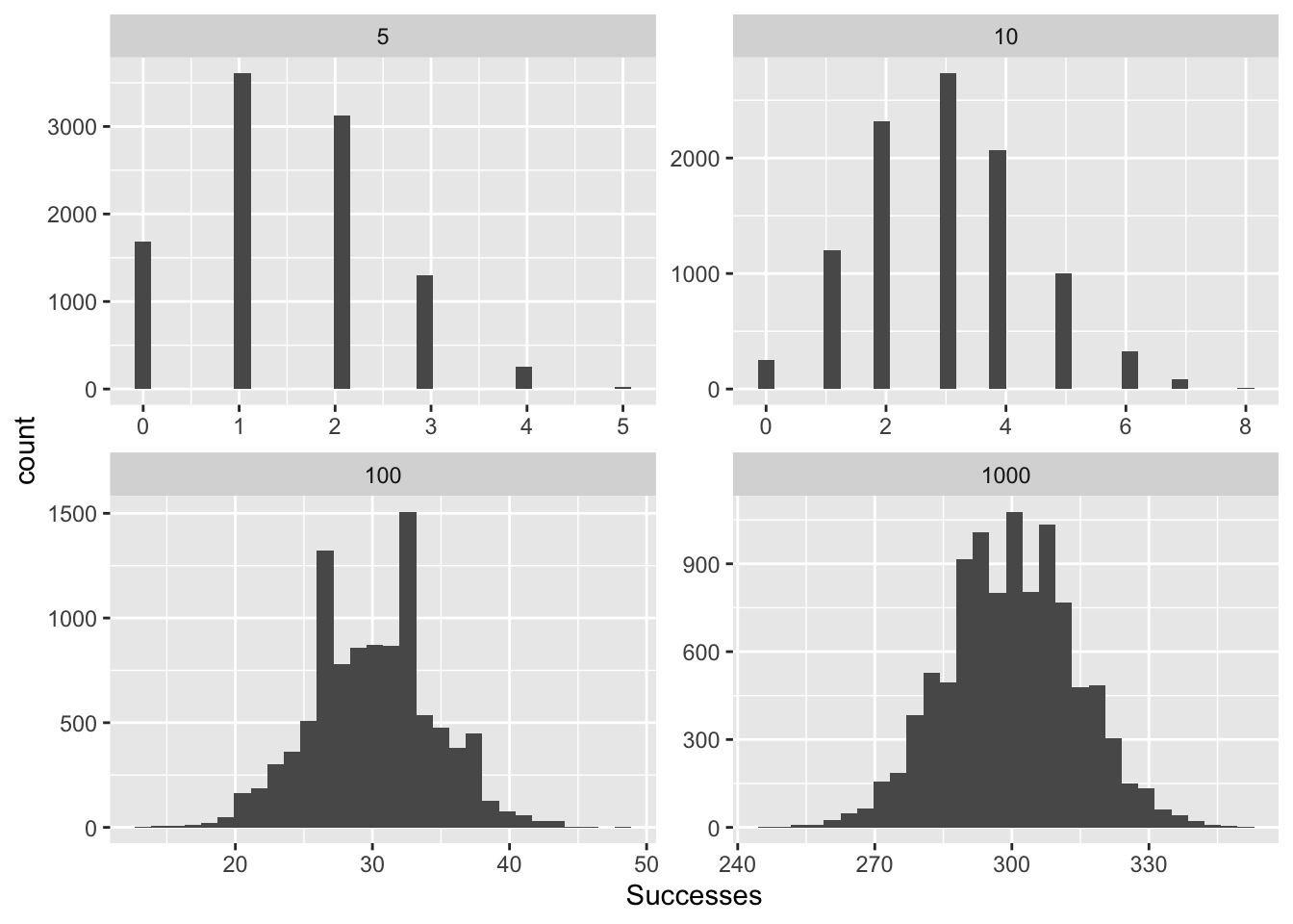
dbinom(3, 10, .3)## [1] 0.2668279pbinom(3, 10, .3)## [1] 0.6496107dbinom(1:10, 10, .3)## [1] 0.1210608210 0.2334744405 0.2668279320 0.2001209490 0.1029193452 0.0367569090 0.0090016920
## [8] 0.0014467005 0.0001377810 0.0000059049pbinom(1:10, 10, .3)## [1] 0.1493083 0.3827828 0.6496107 0.8497317 0.9526510 0.9894079 0.9984096 0.9998563 0.9999941
## [10] 1.0000000qbinom(p=0.2668279, 10, 0.3)## [1] 2dbinom(3, 10, 0.3)## [1] 0.2668279qbinom(p=c(.3, .35, .4, .5, .6), 10, .3)## [1] 2 2 3 3 3qnorm(0.975, 0, 1)## [1] 1.959964#poisson model
# E(dependent variable)= beta * IV
#Poisson distribution
pois1 <- rpois(10000, 1)
hist(pois1)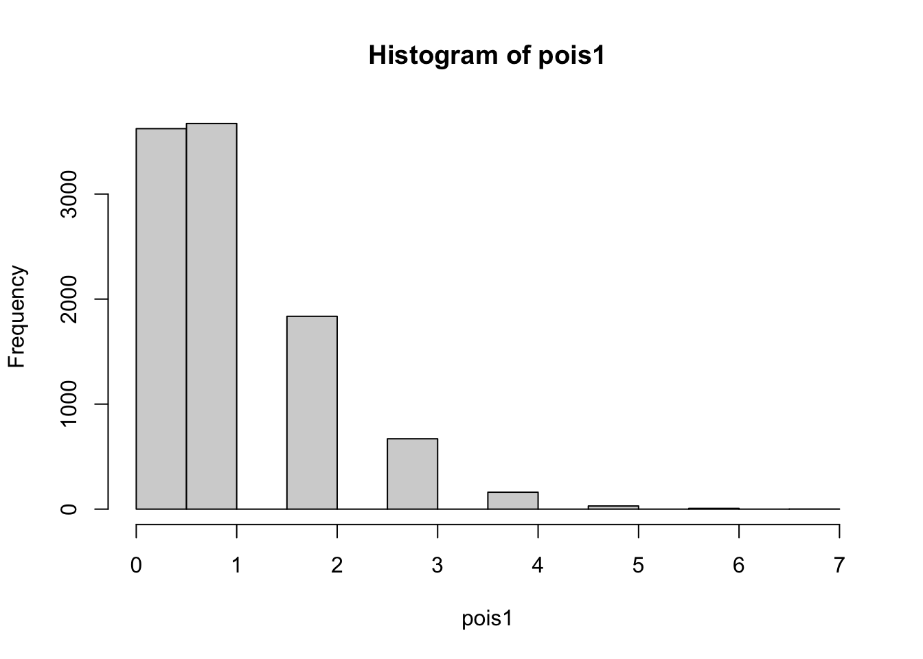
pois2 <- rpois(10000, 2)
max(pois2)
## [1] 9pois5 <- rpois(10000,5)
pois10 <- rpois(10000,10)
pois20 <- rpois(10000,20)
pois <- data.frame(Lambda.1=pois1, Lambda.2=pois2, Lambda.5=pois5,
Lambda.10=pois10, Lambda.20=pois20)
head(pois)## Lambda.1 Lambda.2 Lambda.5 Lambda.10 Lambda.20
## 1 1 2 4 12 22
## 2 1 2 5 5 19
## 3 2 3 8 10 20
## 4 2 1 4 8 29
## 5 0 2 6 8 14
## 6 3 4 6 7 13dim(pois)## [1] 10000 5library(reshape2)
pois <- melt(data = pois, variable.name = "Lambda", value.name = "x")## No id variables; using all as measure variableshead(pois)## Lambda x
## 1 Lambda.1 1
## 2 Lambda.1 1
## 3 Lambda.1 2
## 4 Lambda.1 2
## 5 Lambda.1 0
## 6 Lambda.1 3tail(pois)## Lambda x
## 49995 Lambda.20 15
## 49996 Lambda.20 22
## 49997 Lambda.20 21
## 49998 Lambda.20 21
## 49999 Lambda.20 15
## 50000 Lambda.20 19dim(pois)## [1] 50000 2#"+" keeps all numbers
pois$Lambda <- as.factor(as.numeric(str_extract(string = pois$Lambda,
pattern = "\\d+")))
head(pois)## Lambda x
## 1 1 1
## 2 1 1
## 3 1 2
## 4 1 2
## 5 1 0
## 6 1 3tail(pois)## Lambda x
## 49995 20 15
## 49996 20 22
## 49997 20 21
## 49998 20 21
## 49999 20 15
## 50000 20 19ggplot(pois, aes(x=x))+
geom_histogram(binwidth = 1)+
facet_wrap(~Lambda)+
ggtitle("Probability Mass Function")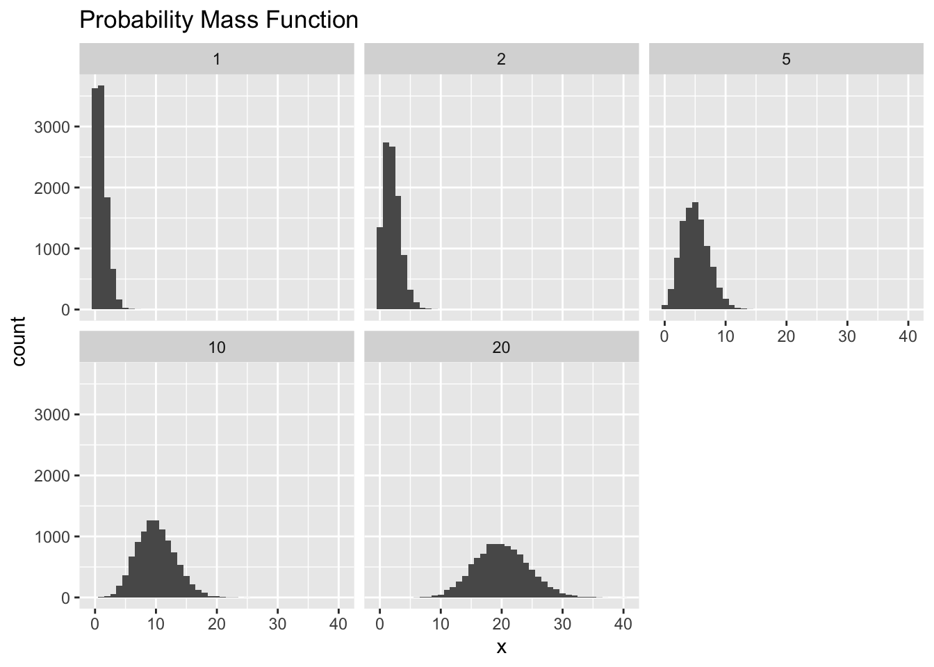
ggplot(pois, aes(x=x))+
  geom_density(aes(group=Lambda, color=Lambda, fill=Lambda),
               adjust=4, alpha=.5)+
  #scale_color_discrete()+
  #scale_fill_discrete()+
  ggtitle("Probability Mass Function")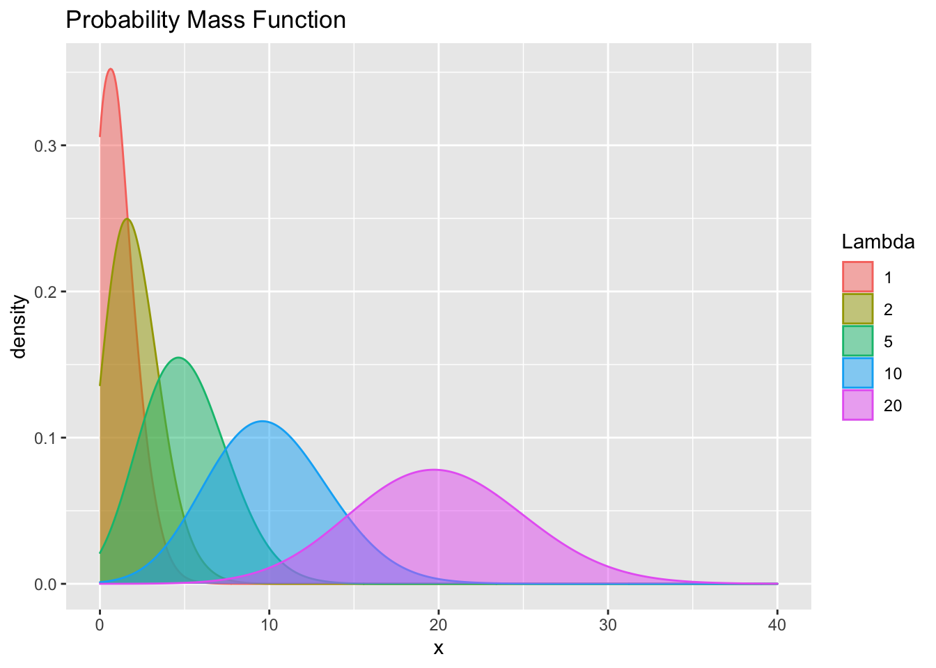
?geom_density
#alpha adjusts transparency
#adjust changes the bandwidch