8 Week 7 : The dplyr package

8.1 What is dplyr?

• When you import your own data into R (probably using the readr package in tidyverse), it is rare that you get the data in the desired form you need for your data visualization and data modeling. The dplyr package provides a set of functions to transform or manipulate your data into the right form you need.

• The official tidyverse website (https://dplyr.tidyverse.org/index.html) introduces the dplyr package as follows:

"dplyr is a grammar of data manipulation, providing a consistent set of verbs that help you solve the most common data manipulation challenges:

• mutate() adds new variables that are functions of existing variables
• select() picks variables based on their names.
• filter() picks cases based on their values.
• summarise() reduces multiple values down to a single summary.
• arrange() changes the ordering of the rows.

These all combine naturally with group_by() which allows you to perform any operation “by group”. You can learn more about them in vignette("dplyr"). As well as these single-table verbs, dplyr also provides a variety of two-table verbs, which you can learn about in vignette("two-table").

If you are new to dplyr, the best place to start is the data transformation chapter in R for data science."

• usage
  • verb(a data frame, what to do with the data frame)
  • e.g., filter(flights, month == 1) # filter the flights data frame to select all flights that departed on Jan. 

8.2 Cheat Sheet

• The cheatsheet for the dplyr package provides nice diagrams illustrating the functionality of various functions in the dplyr package.

8.3 Tibbles

• In Base R, we often use a data frame to store our data. A tibble is the tidyverse version of the data frame in Base R. Tidyverse functions take both the data frame and tibble. Often you may want to explicitly convert a data frame to a tibble using as_tibble():

# iris is a data frame in Base R
as_tibble(iris)

## # A tibble: 150 x 5
##    Sepal.Length Sepal.Width Petal.Length Petal.Width Species
##           <dbl>       <dbl>        <dbl>       <dbl> <fct>  
##  1          5.1         3.5          1.4         0.2 setosa 
##  2          4.9         3            1.4         0.2 setosa 
##  3          4.7         3.2          1.3         0.2 setosa 
##  4          4.6         3.1          1.5         0.2 setosa 
##  5          5           3.6          1.4         0.2 setosa 
##  6          5.4         3.9          1.7         0.4 setosa 
##  7          4.6         3.4          1.4         0.3 setosa 
##  8          5           3.4          1.5         0.2 setosa 
##  9          4.4         2.9          1.4         0.2 setosa 
## 10          4.9         3.1          1.5         0.1 setosa 
## # ... with 140 more rows

For more details about a tibble, you can check here.

8.4 Select columns with select()

• select() subsets columns

# you need the `nycflight13` package to use `flights` data
library(nycflights13)

# names() displays column names
names(flights)

##  [1] "year"           "month"          "day"            "dep_time"      
##  [5] "sched_dep_time" "dep_delay"      "arr_time"       "sched_arr_time"
##  [9] "arr_delay"      "carrier"        "flight"         "tailnum"       
## [13] "origin"         "dest"           "air_time"       "distance"      
## [17] "hour"           "minute"         "time_hour"

# select columns by names
select(flights, year, month, day)

## # A tibble: 336,776 x 3
##     year month   day
##    <int> <int> <int>
##  1  2013     1     1
##  2  2013     1     1
##  3  2013     1     1
##  4  2013     1     1
##  5  2013     1     1
##  6  2013     1     1
##  7  2013     1     1
##  8  2013     1     1
##  9  2013     1     1
## 10  2013     1     1
## # ... with 336,766 more rows

• Tidy selection provides many different ways for selecting variables. You can find more details about the tidy selection here.

• : for selecting a range of consecutive variables

# select all columns between year and day (inclusive)
select(flights, year:day)

## # A tibble: 336,776 x 3
##     year month   day
##    <int> <int> <int>
##  1  2013     1     1
##  2  2013     1     1
##  3  2013     1     1
##  4  2013     1     1
##  5  2013     1     1
##  6  2013     1     1
##  7  2013     1     1
##  8  2013     1     1
##  9  2013     1     1
## 10  2013     1     1
## # ... with 336,766 more rows

• ! for taking the complement of a set of variables.

# select all columns between year and day (inclusive)
select(flights, !(year:day))

## # A tibble: 336,776 x 16
##    dep_time sched_dep_time dep_delay arr_time sched_arr_time arr_delay carrier
##       <int>          <int>     <dbl>    <int>          <int>     <dbl> <chr>  
##  1      517            515         2      830            819        11 UA     
##  2      533            529         4      850            830        20 UA     
##  3      542            540         2      923            850        33 AA     
##  4      544            545        -1     1004           1022       -18 B6     
##  5      554            600        -6      812            837       -25 DL     
##  6      554            558        -4      740            728        12 UA     
##  7      555            600        -5      913            854        19 B6     
##  8      557            600        -3      709            723       -14 EV     
##  9      557            600        -3      838            846        -8 B6     
## 10      558            600        -2      753            745         8 AA     
## # ... with 336,766 more rows, and 9 more variables: flight <int>,
## #   tailnum <chr>, origin <chr>, dest <chr>, air_time <dbl>, distance <dbl>,
## #   hour <dbl>, minute <dbl>, time_hour <dttm>

• Selection helper functions select variables by matching patterns in their names:

  • starts_with(): Starts with a prefix.

  • ends_with(): Ends with a suffix.

  • contains(): Contains a literal string.

  • matches(): Matches a regular expression.

  • num_range(): Matches a numerical range like x01, x02, x03.

# select all columns starts with "dep"
select(flights, starts_with("dep"))

## # A tibble: 336,776 x 2
##    dep_time dep_delay
##       <int>     <dbl>
##  1      517         2
##  2      533         4
##  3      542         2
##  4      544        -1
##  5      554        -6
##  6      554        -4
##  7      555        -5
##  8      557        -3
##  9      557        -3
## 10      558        -2
## # ... with 336,766 more rows

# select all columns ends with "time"
select(flights, ends_with("time"))

## # A tibble: 336,776 x 5
##    dep_time sched_dep_time arr_time sched_arr_time air_time
##       <int>          <int>    <int>          <int>    <dbl>
##  1      517            515      830            819      227
##  2      533            529      850            830      227
##  3      542            540      923            850      160
##  4      544            545     1004           1022      183
##  5      554            600      812            837      116
##  6      554            558      740            728      150
##  7      555            600      913            854      158
##  8      557            600      709            723       53
##  9      557            600      838            846      140
## 10      558            600      753            745      138
## # ... with 336,766 more rows

# select all columns contains "time"
select(flights, contains("time"))

## # A tibble: 336,776 x 6
##    dep_time sched_dep_time arr_time sched_arr_time air_time time_hour          
##       <int>          <int>    <int>          <int>    <dbl> <dttm>             
##  1      517            515      830            819      227 2013-01-01 05:00:00
##  2      533            529      850            830      227 2013-01-01 05:00:00
##  3      542            540      923            850      160 2013-01-01 05:00:00
##  4      544            545     1004           1022      183 2013-01-01 05:00:00
##  5      554            600      812            837      116 2013-01-01 06:00:00
##  6      554            558      740            728      150 2013-01-01 05:00:00
##  7      555            600      913            854      158 2013-01-01 06:00:00
##  8      557            600      709            723       53 2013-01-01 06:00:00
##  9      557            600      838            846      140 2013-01-01 06:00:00
## 10      558            600      753            745      138 2013-01-01 06:00:00
## # ... with 336,766 more rows

# select all columns starts with "dep", contains "time", and between year and day (inclusive)
select(flights, starts_with("dep"), contains("time"), year:day)

## # A tibble: 336,776 x 10
##    dep_time dep_delay sched_dep_time arr_time sched_arr_time air_time
##       <int>     <dbl>          <int>    <int>          <int>    <dbl>
##  1      517         2            515      830            819      227
##  2      533         4            529      850            830      227
##  3      542         2            540      923            850      160
##  4      544        -1            545     1004           1022      183
##  5      554        -6            600      812            837      116
##  6      554        -4            558      740            728      150
##  7      555        -5            600      913            854      158
##  8      557        -3            600      709            723       53
##  9      557        -3            600      838            846      140
## 10      558        -2            600      753            745      138
## # ... with 336,766 more rows, and 4 more variables: time_hour <dttm>,
## #   year <int>, month <int>, day <int>

# select columns 1,3,5
select(flights, c(1,3,5))

## # A tibble: 336,776 x 3
##     year   day sched_dep_time
##    <int> <int>          <int>
##  1  2013     1            515
##  2  2013     1            529
##  3  2013     1            540
##  4  2013     1            545
##  5  2013     1            600
##  6  2013     1            558
##  7  2013     1            600
##  8  2013     1            600
##  9  2013     1            600
## 10  2013     1            600
## # ... with 336,766 more rows

# billboard is a dataset in the tidyverse package
# billboard contains song rankings for billboard top 100 in 2000
billboard

## # A tibble: 317 x 79
##    artist track date.entered   wk1   wk2   wk3   wk4   wk5   wk6   wk7   wk8
##    <chr>  <chr> <date>       <dbl> <dbl> <dbl> <dbl> <dbl> <dbl> <dbl> <dbl>
##  1 2 Pac  Baby~ 2000-02-26      87    82    72    77    87    94    99    NA
##  2 2Ge+h~ The ~ 2000-09-02      91    87    92    NA    NA    NA    NA    NA
##  3 3 Doo~ Kryp~ 2000-04-08      81    70    68    67    66    57    54    53
##  4 3 Doo~ Loser 2000-10-21      76    76    72    69    67    65    55    59
##  5 504 B~ Wobb~ 2000-04-15      57    34    25    17    17    31    36    49
##  6 98^0   Give~ 2000-08-19      51    39    34    26    26    19     2     2
##  7 A*Tee~ Danc~ 2000-07-08      97    97    96    95   100    NA    NA    NA
##  8 Aaliy~ I Do~ 2000-01-29      84    62    51    41    38    35    35    38
##  9 Aaliy~ Try ~ 2000-03-18      59    53    38    28    21    18    16    14
## 10 Adams~ Open~ 2000-08-26      76    76    74    69    68    67    61    58
## # ... with 307 more rows, and 68 more variables: wk9 <dbl>, wk10 <dbl>,
## #   wk11 <dbl>, wk12 <dbl>, wk13 <dbl>, wk14 <dbl>, wk15 <dbl>, wk16 <dbl>,
## #   wk17 <dbl>, wk18 <dbl>, wk19 <dbl>, wk20 <dbl>, wk21 <dbl>, wk22 <dbl>,
## #   wk23 <dbl>, wk24 <dbl>, wk25 <dbl>, wk26 <dbl>, wk27 <dbl>, wk28 <dbl>,
## #   wk29 <dbl>, wk30 <dbl>, wk31 <dbl>, wk32 <dbl>, wk33 <dbl>, wk34 <dbl>,
## #   wk35 <dbl>, wk36 <dbl>, wk37 <dbl>, wk38 <dbl>, wk39 <dbl>, wk40 <dbl>,
## #   wk41 <dbl>, wk42 <dbl>, wk43 <dbl>, wk44 <dbl>, wk45 <dbl>, wk46 <dbl>,
## #   wk47 <dbl>, wk48 <dbl>, wk49 <dbl>, wk50 <dbl>, wk51 <dbl>, wk52 <dbl>,
## #   wk53 <dbl>, wk54 <dbl>, wk55 <dbl>, wk56 <dbl>, wk57 <dbl>, wk58 <dbl>,
## #   wk59 <dbl>, wk60 <dbl>, wk61 <dbl>, wk62 <dbl>, wk63 <dbl>, wk64 <dbl>,
## #   wk65 <dbl>, wk66 <lgl>, wk67 <lgl>, wk68 <lgl>, wk69 <lgl>, wk70 <lgl>,
## #   wk71 <lgl>, wk72 <lgl>, wk73 <lgl>, wk74 <lgl>, wk75 <lgl>, wk76 <lgl>

# names() returns columns of a dataset
names(billboard)

##  [1] "artist"       "track"        "date.entered" "wk1"          "wk2"         
##  [6] "wk3"          "wk4"          "wk5"          "wk6"          "wk7"         
## [11] "wk8"          "wk9"          "wk10"         "wk11"         "wk12"        
## [16] "wk13"         "wk14"         "wk15"         "wk16"         "wk17"        
## [21] "wk18"         "wk19"         "wk20"         "wk21"         "wk22"        
## [26] "wk23"         "wk24"         "wk25"         "wk26"         "wk27"        
## [31] "wk28"         "wk29"         "wk30"         "wk31"         "wk32"        
## [36] "wk33"         "wk34"         "wk35"         "wk36"         "wk37"        
## [41] "wk38"         "wk39"         "wk40"         "wk41"         "wk42"        
## [46] "wk43"         "wk44"         "wk45"         "wk46"         "wk47"        
## [51] "wk48"         "wk49"         "wk50"         "wk51"         "wk52"        
## [56] "wk53"         "wk54"         "wk55"         "wk56"         "wk57"        
## [61] "wk58"         "wk59"         "wk60"         "wk61"         "wk62"        
## [66] "wk63"         "wk64"         "wk65"         "wk66"         "wk67"        
## [71] "wk68"         "wk69"         "wk70"         "wk71"         "wk72"        
## [76] "wk73"         "wk74"         "wk75"         "wk76"

select(billboard, num_range("wk", 20:23))

## # A tibble: 317 x 4
##     wk20  wk21  wk22  wk23
##    <dbl> <dbl> <dbl> <dbl>
##  1    NA    NA    NA    NA
##  2    NA    NA    NA    NA
##  3    14    12     7     6
##  4    70    NA    NA    NA
##  5    NA    NA    NA    NA
##  6    94    NA    NA    NA
##  7    NA    NA    NA    NA
##  8    86    NA    NA    NA
##  9     4     5     5     6
## 10    89    NA    NA    NA
## # ... with 307 more rows

8.5 Filter rows with filter()

• filter() subsets observations based on their values

• multiple arguments to filter are combined using logical operators

  • & and
  • | or
  • ! not

• By default, multiple conditions are combined with &

# filter the flights departed on Jan 1.
# Here month == 1 & day == 1    
filter(flights, month == 1, day == 1) 

## # A tibble: 842 x 19
##     year month   day dep_time sched_dep_time dep_delay arr_time sched_arr_time
##    <int> <int> <int>    <int>          <int>     <dbl>    <int>          <int>
##  1  2013     1     1      517            515         2      830            819
##  2  2013     1     1      533            529         4      850            830
##  3  2013     1     1      542            540         2      923            850
##  4  2013     1     1      544            545        -1     1004           1022
##  5  2013     1     1      554            600        -6      812            837
##  6  2013     1     1      554            558        -4      740            728
##  7  2013     1     1      555            600        -5      913            854
##  8  2013     1     1      557            600        -3      709            723
##  9  2013     1     1      557            600        -3      838            846
## 10  2013     1     1      558            600        -2      753            745
## # ... with 832 more rows, and 11 more variables: arr_delay <dbl>,
## #   carrier <chr>, flight <int>, tailnum <chr>, origin <chr>, dest <chr>,
## #   air_time <dbl>, distance <dbl>, hour <dbl>, minute <dbl>, time_hour <dttm>

# filter the flights departed on Nov or Dec
filter(flights, month == 11 | month == 12) 

## # A tibble: 55,403 x 19
##     year month   day dep_time sched_dep_time dep_delay arr_time sched_arr_time
##    <int> <int> <int>    <int>          <int>     <dbl>    <int>          <int>
##  1  2013    11     1        5           2359         6      352            345
##  2  2013    11     1       35           2250       105      123           2356
##  3  2013    11     1      455            500        -5      641            651
##  4  2013    11     1      539            545        -6      856            827
##  5  2013    11     1      542            545        -3      831            855
##  6  2013    11     1      549            600       -11      912            923
##  7  2013    11     1      550            600       -10      705            659
##  8  2013    11     1      554            600        -6      659            701
##  9  2013    11     1      554            600        -6      826            827
## 10  2013    11     1      554            600        -6      749            751
## # ... with 55,393 more rows, and 11 more variables: arr_delay <dbl>,
## #   carrier <chr>, flight <int>, tailnum <chr>, origin <chr>, dest <chr>,
## #   air_time <dbl>, distance <dbl>, hour <dbl>, minute <dbl>, time_hour <dttm>

# filter the flights to IAH
filter(flights, dest == "IAH") 

## # A tibble: 7,198 x 19
##     year month   day dep_time sched_dep_time dep_delay arr_time sched_arr_time
##    <int> <int> <int>    <int>          <int>     <dbl>    <int>          <int>
##  1  2013     1     1      517            515         2      830            819
##  2  2013     1     1      533            529         4      850            830
##  3  2013     1     1      623            627        -4      933            932
##  4  2013     1     1      728            732        -4     1041           1038
##  5  2013     1     1      739            739         0     1104           1038
##  6  2013     1     1      908            908         0     1228           1219
##  7  2013     1     1     1028           1026         2     1350           1339
##  8  2013     1     1     1044           1045        -1     1352           1351
##  9  2013     1     1     1114            900       134     1447           1222
## 10  2013     1     1     1205           1200         5     1503           1505
## # ... with 7,188 more rows, and 11 more variables: arr_delay <dbl>,
## #   carrier <chr>, flight <int>, tailnum <chr>, origin <chr>, dest <chr>,
## #   air_time <dbl>, distance <dbl>, hour <dbl>, minute <dbl>, time_hour <dttm>

# filter the flights with arr_delay <= 120 or dep_delay > 120
filter(flights, arr_delay <= 120 | dep_delay > 120) 

## # A tibble: 325,773 x 19
##     year month   day dep_time sched_dep_time dep_delay arr_time sched_arr_time
##    <int> <int> <int>    <int>          <int>     <dbl>    <int>          <int>
##  1  2013     1     1      517            515         2      830            819
##  2  2013     1     1      533            529         4      850            830
##  3  2013     1     1      542            540         2      923            850
##  4  2013     1     1      544            545        -1     1004           1022
##  5  2013     1     1      554            600        -6      812            837
##  6  2013     1     1      554            558        -4      740            728
##  7  2013     1     1      555            600        -5      913            854
##  8  2013     1     1      557            600        -3      709            723
##  9  2013     1     1      557            600        -3      838            846
## 10  2013     1     1      558            600        -2      753            745
## # ... with 325,763 more rows, and 11 more variables: arr_delay <dbl>,
## #   carrier <chr>, flight <int>, tailnum <chr>, origin <chr>, dest <chr>,
## #   air_time <dbl>, distance <dbl>, hour <dbl>, minute <dbl>, time_hour <dttm>

8.6 Add new variables with mutate()

• mutate() create a new variable.

mutate(flights, gain = arr_delay - dep_delay, hours = air_time / 60, gain_per_hour = gain / hours)

## # A tibble: 336,776 x 22
##     year month   day dep_time sched_dep_time dep_delay arr_time sched_arr_time
##    <int> <int> <int>    <int>          <int>     <dbl>    <int>          <int>
##  1  2013     1     1      517            515         2      830            819
##  2  2013     1     1      533            529         4      850            830
##  3  2013     1     1      542            540         2      923            850
##  4  2013     1     1      544            545        -1     1004           1022
##  5  2013     1     1      554            600        -6      812            837
##  6  2013     1     1      554            558        -4      740            728
##  7  2013     1     1      555            600        -5      913            854
##  8  2013     1     1      557            600        -3      709            723
##  9  2013     1     1      557            600        -3      838            846
## 10  2013     1     1      558            600        -2      753            745
## # ... with 336,766 more rows, and 14 more variables: arr_delay <dbl>,
## #   carrier <chr>, flight <int>, tailnum <chr>, origin <chr>, dest <chr>,
## #   air_time <dbl>, distance <dbl>, hour <dbl>, minute <dbl>, time_hour <dttm>,
## #   gain <dbl>, hours <dbl>, gain_per_hour <dbl>

• mutate() executes the transformations iteratively so that later transformations can use the columns created by earlier transformations.

mutate(flights, gain = arr_delay - dep_delay, hours = air_time / 60, gain_per_hour = gain / hours)

## # A tibble: 336,776 x 22
##     year month   day dep_time sched_dep_time dep_delay arr_time sched_arr_time
##    <int> <int> <int>    <int>          <int>     <dbl>    <int>          <int>
##  1  2013     1     1      517            515         2      830            819
##  2  2013     1     1      533            529         4      850            830
##  3  2013     1     1      542            540         2      923            850
##  4  2013     1     1      544            545        -1     1004           1022
##  5  2013     1     1      554            600        -6      812            837
##  6  2013     1     1      554            558        -4      740            728
##  7  2013     1     1      555            600        -5      913            854
##  8  2013     1     1      557            600        -3      709            723
##  9  2013     1     1      557            600        -3      838            846
## 10  2013     1     1      558            600        -2      753            745
## # ... with 336,766 more rows, and 14 more variables: arr_delay <dbl>,
## #   carrier <chr>, flight <int>, tailnum <chr>, origin <chr>, dest <chr>,
## #   air_time <dbl>, distance <dbl>, hour <dbl>, minute <dbl>, time_hour <dttm>,
## #   gain <dbl>, hours <dbl>, gain_per_hour <dbl>

• transmute() creates a new variable but drops others.

transmute(flights, gain = arr_delay - dep_delay, hours = air_time / 60, gain_per_hour = gain / hours)

## # A tibble: 336,776 x 3
##     gain hours gain_per_hour
##    <dbl> <dbl>         <dbl>
##  1     9 3.78           2.38
##  2    16 3.78           4.23
##  3    31 2.67          11.6 
##  4   -17 3.05          -5.57
##  5   -19 1.93          -9.83
##  6    16 2.5            6.4 
##  7    24 2.63           9.11
##  8   -11 0.883        -12.5 
##  9    -5 2.33          -2.14
## 10    10 2.3            4.35
## # ... with 336,766 more rows

• The scoped variant of mutate() and transmute() help us to apply the same transformation to multiple variables.

  • mutate_all() and transmute_all() affect every variable

  • mutate_at() and transmute_at() affect variables selected with a character vector

  • mutate_if() and transmute_if() affect variables selected with a predicate function (a function that returns TRUE or FALSE)

head(iris)

##   Sepal.Length Sepal.Width Petal.Length Petal.Width Species
## 1          5.1         3.5          1.4         0.2  setosa
## 2          4.9         3.0          1.4         0.2  setosa
## 3          4.7         3.2          1.3         0.2  setosa
## 4          4.6         3.1          1.5         0.2  setosa
## 5          5.0         3.6          1.4         0.2  setosa
## 6          5.4         3.9          1.7         0.4  setosa

# apply log() to the columns that contain "Sepal"
mutated <- mutate_at(iris, vars(contains("Sepal")), log)
head(mutated) 

##   Sepal.Length Sepal.Width Petal.Length Petal.Width Species
## 1     1.629241    1.252763          1.4         0.2  setosa
## 2     1.589235    1.098612          1.4         0.2  setosa
## 3     1.547563    1.163151          1.3         0.2  setosa
## 4     1.526056    1.131402          1.5         0.2  setosa
## 5     1.609438    1.280934          1.4         0.2  setosa
## 6     1.686399    1.360977          1.7         0.4  setosa

# apply log() to the numeric columns
mutated <- mutate_if(iris, is.numeric, log)
head(mutated)

##   Sepal.Length Sepal.Width Petal.Length Petal.Width Species
## 1     1.629241    1.252763    0.3364722  -1.6094379  setosa
## 2     1.589235    1.098612    0.3364722  -1.6094379  setosa
## 3     1.547563    1.163151    0.2623643  -1.6094379  setosa
## 4     1.526056    1.131402    0.4054651  -1.6094379  setosa
## 5     1.609438    1.280934    0.3364722  -1.6094379  setosa
## 6     1.686399    1.360977    0.5306283  -0.9162907  setosa

• You will find more details about the scoped variants of mutate() and transmute() here.

• Tidyverse changes rapidly. To indicate the lifecycle of packages (or functions), Tidyverse uses the lifecycle badges.

• Now, across() supersedes the family of “scoped variants” like summarise_at(), summarise_if(), and summarise_all(). It means that you will see more across() and less _at(), _if(), _all() functions in the future.

  • You can check the following links for more details about across()
    • https://dplyr.tidyverse.org/articles/colwise.html
    • https://www.tidyverse.org/blog/2020/04/dplyr-1-0-0-colwise/

8.7 Arrange rows with arrange()

• arrange() reorders rows in ascending order by default
  • use desc() to order in descending order

arrange(flights, year, month, day)

## # A tibble: 336,776 x 19
##     year month   day dep_time sched_dep_time dep_delay arr_time sched_arr_time
##    <int> <int> <int>    <int>          <int>     <dbl>    <int>          <int>
##  1  2013     1     1      517            515         2      830            819
##  2  2013     1     1      533            529         4      850            830
##  3  2013     1     1      542            540         2      923            850
##  4  2013     1     1      544            545        -1     1004           1022
##  5  2013     1     1      554            600        -6      812            837
##  6  2013     1     1      554            558        -4      740            728
##  7  2013     1     1      555            600        -5      913            854
##  8  2013     1     1      557            600        -3      709            723
##  9  2013     1     1      557            600        -3      838            846
## 10  2013     1     1      558            600        -2      753            745
## # ... with 336,766 more rows, and 11 more variables: arr_delay <dbl>,
## #   carrier <chr>, flight <int>, tailnum <chr>, origin <chr>, dest <chr>,
## #   air_time <dbl>, distance <dbl>, hour <dbl>, minute <dbl>, time_hour <dttm>

arrange(flights, desc(month))

## # A tibble: 336,776 x 19
##     year month   day dep_time sched_dep_time dep_delay arr_time sched_arr_time
##    <int> <int> <int>    <int>          <int>     <dbl>    <int>          <int>
##  1  2013    12     1       13           2359        14      446            445
##  2  2013    12     1       17           2359        18      443            437
##  3  2013    12     1      453            500        -7      636            651
##  4  2013    12     1      520            515         5      749            808
##  5  2013    12     1      536            540        -4      845            850
##  6  2013    12     1      540            550       -10     1005           1027
##  7  2013    12     1      541            545        -4      734            755
##  8  2013    12     1      546            545         1      826            835
##  9  2013    12     1      549            600       -11      648            659
## 10  2013    12     1      550            600       -10      825            854
## # ... with 336,766 more rows, and 11 more variables: arr_delay <dbl>,
## #   carrier <chr>, flight <int>, tailnum <chr>, origin <chr>, dest <chr>,
## #   air_time <dbl>, distance <dbl>, hour <dbl>, minute <dbl>, time_hour <dttm>

8.8 Grouped summaries with summarize()

• summarize() collapses a tibble to a single row for summary (imagine the sum and average function in Excel)
• summarize() is not terribly useful unless we pair it with group_by().
• group_by() takes an existing tibble and converts it into a grouped tibble where operations are performed “by group”.
• Using group_by(), most data operations are done on groups defined by variables.
• Together group_by(), summarize() will produce one row for each group
• group_by() and summarize() provide one of the tools that you’ll use most commonly when working with dplyr: grouped summaries.
• summarize(data, …)
  • … = Name-value pairs of summary functions. The name will be the name of the variable in the result. The value should be an expression that returns a single value like min(x), n(), or sum(is.na(y)).
• Summary functions takes a vector as an input and return a single value as an output.
  • Counts
  • Locations
  • Position/

# name = delay, value = mean(dep_delay, na.rm = TRUE)
summarize(flights, delay_mean = mean(dep_delay, na.rm = TRUE), delay_sd = sd(dep_delay, na.rm = TRUE))

## # A tibble: 1 x 2
##   delay_mean delay_sd
##        <dbl>    <dbl>
## 1       12.6     40.2

# Together `group_by()`, `summarize()` will produce one row for each group
by_day <- group_by(flights, year, month, day) 
summarize(by_day, delay = mean(dep_delay, na.rm = TRUE))

## `summarise()` regrouping output by 'year', 'month' (override with `.groups` argument)

## # A tibble: 365 x 4
## # Groups:   year, month [12]
##     year month   day delay
##    <int> <int> <int> <dbl>
##  1  2013     1     1 11.5 
##  2  2013     1     2 13.9 
##  3  2013     1     3 11.0 
##  4  2013     1     4  8.95
##  5  2013     1     5  5.73
##  6  2013     1     6  7.15
##  7  2013     1     7  5.42
##  8  2013     1     8  2.55
##  9  2013     1     9  2.28
## 10  2013     1    10  2.84
## # ... with 355 more rows

8.9 The pipe operator %>%

• You will find %>% in almost all tidyverse codes. The pipe operator %>% from the magrittr package was developed to help you write code that is easier to read and understand or to enhance the readability of your code. Since the tidyverse automatically load %>%, you don’t need to manually load the magrittr package to use %>%. Here’s what the pipe operator %>% does:

  • x %>% f(y) turns into f(x, y)
  • x %>% f(y) %>% g(z) turns into g(f(x,y), z)

• The pipe operator %>% focuses on the the transformations, not what’s being transformed. You can read it as a series of imperative statements: do f() and “then” do g(). A good way to pronounce %>% when reading the code is “then”.

• Let’s see a concrete example.

by_dest <- group_by(flights, dest) 
delay <- summarize(by_dest, count = n(), dist = mean(distance, na.rm = TRUE), delay = mean( arr_delay, na.rm = TRUE)) 
delay <- filter(delay, count > 20, dest != "HNL") 
delay

## # A tibble: 96 x 4
##    dest  count  dist delay
##    <chr> <int> <dbl> <dbl>
##  1 ABQ     254 1826   4.38
##  2 ACK     265  199   4.85
##  3 ALB     439  143  14.4 
##  4 ATL   17215  757. 11.3 
##  5 AUS    2439 1514.  6.02
##  6 AVL     275  584.  8.00
##  7 BDL     443  116   7.05
##  8 BGR     375  378   8.03
##  9 BHM     297  866. 16.9 
## 10 BNA    6333  758. 11.8 
## # ... with 86 more rows

# It looks like delays increase with distance up to ~ 750 miles and then decrease. Maybe as flights get longer there's more ability to make up delays in the air? 
ggplot(data = delay, mapping = aes(x = dist, y = delay)) + 
  geom_point( aes( size = count), alpha = 1/3) + 
  geom_smooth(se = FALSE)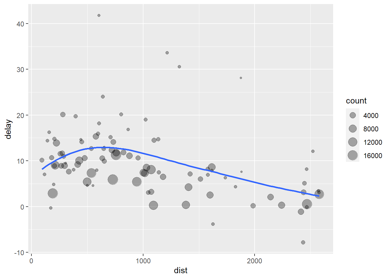

• The code above is a little frustrating to write because we have to give each intermediate data frame a name, even though we don’t care about it. Naming things is hard, so this slows down our analysis.The code below focuses on the transformations, not what’s being transformed, which makes the code easier to read. You can read it as a series of imperative statements: group, then summarize, then filter, then ggplot. As suggested by this reading, a good way to pronounce %>% when reading code is “then.”

flights %>% 
  group_by(dest) %>% 
  summarize(count = n(), dist = mean( distance, na.rm = TRUE), delay = mean(arr_delay, na.rm = TRUE)) %>%
  filter(count > 20, dest != "HNL") %>% 
  ggplot(mapping = aes(x = dist, y = delay)) + 
    geom_point(aes(size = count), alpha = 1/3) + 
    geom_smooth(se = FALSE)

8.10 Style Guide

• It is important to make your codes easy to read by human (especially you). In order to enhance the readability of your codes, it is often recommended to
  • add comments (# in R)
  • follow programming style guides
• Programming style guides are a set of guidelines used when writing the source code for a specific programming language. Your R codes will still work even though you don’t follow the style guide. However, style guides will enhance the readability of your code. R has a couple of style guides:
  • Google’s R Style Guide
  • The tidyverse style guide

8.11 Grouped summaries with summarize() (continue)

• iris is a built-in dataset in R and gives the measurements in centimeters of the variables sepal length and width and petal length and width, respectively, for 50 flowers from each of 3 species of iris. The species are Iris setosa, versicolor, and virginica. You can find the pictures of three species here.

as_tibble(iris)

## # A tibble: 150 x 5
##    Sepal.Length Sepal.Width Petal.Length Petal.Width Species
##           <dbl>       <dbl>        <dbl>       <dbl> <fct>  
##  1          5.1         3.5          1.4         0.2 setosa 
##  2          4.9         3            1.4         0.2 setosa 
##  3          4.7         3.2          1.3         0.2 setosa 
##  4          4.6         3.1          1.5         0.2 setosa 
##  5          5           3.6          1.4         0.2 setosa 
##  6          5.4         3.9          1.7         0.4 setosa 
##  7          4.6         3.4          1.4         0.3 setosa 
##  8          5           3.4          1.5         0.2 setosa 
##  9          4.4         2.9          1.4         0.2 setosa 
## 10          4.9         3.1          1.5         0.1 setosa 
## # ... with 140 more rows

# without the pipe operator %>%
iris_grouped <- group_by(iris, Species) 
summarise_all(iris_grouped, mean)

## # A tibble: 3 x 5
##   Species    Sepal.Length Sepal.Width Petal.Length Petal.Width
##   <fct>             <dbl>       <dbl>        <dbl>       <dbl>
## 1 setosa             5.01        3.43         1.46       0.246
## 2 versicolor         5.94        2.77         4.26       1.33 
## 3 virginica          6.59        2.97         5.55       2.03

# with the pipe operator %>%
# with summarise_all() - superseded by across()
iris %>% 
  group_by(Species) %>%
  summarise_all(mean)

## # A tibble: 3 x 5
##   Species    Sepal.Length Sepal.Width Petal.Length Petal.Width
##   <fct>             <dbl>       <dbl>        <dbl>       <dbl>
## 1 setosa             5.01        3.43         1.46       0.246
## 2 versicolor         5.94        2.77         4.26       1.33 
## 3 virginica          6.59        2.97         5.55       2.03

# with the pipe operator %>%
# selection helper functions are useful for selecting columns
iris %>% 
  group_by(Species) %>%
  summarise(across(starts_with("Sepal"), mean))

## `summarise()` ungrouping output (override with `.groups` argument)

## # A tibble: 3 x 3
##   Species    Sepal.Length Sepal.Width
##   <fct>             <dbl>       <dbl>
## 1 setosa             5.01        3.43
## 2 versicolor         5.94        2.77
## 3 virginica          6.59        2.97

• The High School and Beyond(HSB) dataset is a dataset in the candisc package. The High School and Beyond Project was a longitudinal study of students in the U.S. carried out in 1980 by the National Center for Education Statistics. Data were collected from 58,270 high school students (28,240 seniors and 30,030 sophomores) and 1,015 secondary schools. The HSB data frame is sample of 600 observations, of unknown characteristics, originally taken from Tatsuoka (1988).

# you need a `candisc` package to use the high school and beyond (HSB) data
library(candisc)

# data() loads specific data sets
data(HSB)

# as_tibble() converts a dataframe to a tibble
# a tibble prints the first part of a dataset by default 
# We need head() to prints the first part of a dataframe
HSB_tbl <- as_tibble(HSB)
HSB_tbl

## # A tibble: 600 x 15
##       id gender race  ses   sch   prog    locus concept   mot career  read write
##    <dbl> <fct>  <fct> <fct> <fct> <fct>   <dbl>   <dbl> <dbl> <fct>  <dbl> <dbl>
##  1    55 female hisp~ low   publ~ gene~ -1.78     0.560 1     prof1   28.3  46.3
##  2   114 male   afri~ midd~ publ~ acad~  0.240   -0.350 1     opera~  30.5  35.9
##  3   490 male   white midd~ publ~ voca~ -1.28     0.340 0.330 prof1   31    35.9
##  4    44 female hisp~ low   publ~ voca~  0.220   -0.760 1     servi~  31    41.1
##  5    26 female hisp~ midd~ publ~ acad~  1.12    -0.740 0.670 servi~  31    41.1
##  6   510 male   white midd~ publ~ voca~ -0.860    1.19  0.330 opera~  33.6  28.1
##  7   133 female afri~ low   publ~ voca~ -0.230    0.440 0.330 school  33.6  35.2
##  8   213 female white low   publ~ gene~  0.0400  -0.470 0.670 cleri~  33.6  59.3
##  9   548 female white midd~ priv~ acad~  0.470    0.340 0.670 prof2   33.6  43  
## 10   309 female white high  publ~ gene~  0.320    0.900 0.670 prof2   33.6  51.5
## # ... with 590 more rows, and 3 more variables: math <dbl>, sci <dbl>, ss <dbl>

# names() displays the column names of the HSB data
# ?HSB will give you more details about HSB data
names(HSB_tbl)

##  [1] "id"      "gender"  "race"    "ses"     "sch"     "prog"    "locus"  
##  [8] "concept" "mot"     "career"  "read"    "write"   "math"    "sci"    
## [15] "ss"

str(HSB_tbl)

## tibble [600 x 15] (S3: tbl_df/tbl/data.frame)
##  $ id     : num [1:600] 55 114 490 44 26 510 133 213 548 309 ...
##  $ gender : Factor w/ 2 levels "male","female": 2 1 1 2 2 1 2 2 2 2 ...
##  $ race   : Factor w/ 4 levels "hispanic","asian",..: 1 3 4 1 1 4 3 4 4 4 ...
##  $ ses    : Factor w/ 3 levels "low","middle",..: 1 2 2 1 2 2 1 1 2 3 ...
##  $ sch    : Factor w/ 2 levels "public","private": 1 1 1 1 1 1 1 1 2 1 ...
##  $ prog   : Factor w/ 3 levels "general","academic",..: 1 2 3 3 2 3 3 1 2 1 ...
##  $ locus  : num [1:600] -1.78 0.24 -1.28 0.22 1.12 ...
##  $ concept: num [1:600] 0.56 -0.35 0.34 -0.76 -0.74 ...
##  $ mot    : num [1:600] 1 1 0.33 1 0.67 ...
##  $ career : Factor w/ 17 levels "clerical","craftsman",..: 9 8 9 15 15 8 14 1 10 10 ...
##  $ read   : num [1:600] 28.3 30.5 31 31 31 ...
##  $ write  : num [1:600] 46.3 35.9 35.9 41.1 41.1 ...
##  $ math   : num [1:600] 42.8 36.9 46.1 49.2 36 ...
##  $ sci    : num [1:600] 44.4 33.6 39 33.6 36.9 ...
##  $ ss     : num [1:600] 50.6 40.6 45.6 35.6 45.6 ...

# n() gives the current group size
HSB_tbl %>%
  group_by(race) %>%
  summarise(n = n())

## `summarise()` ungrouping output (override with `.groups` argument)

## # A tibble: 4 x 2
##   race             n
##   <fct>        <int>
## 1 hispanic        71
## 2 asian           34
## 3 african-amer    58
## 4 white          437

# count() counts the unique values of variables
HSB_tbl %>% 
  count(race)

## # A tibble: 4 x 2
##   race             n
##   <fct>        <int>
## 1 hispanic        71
## 2 asian           34
## 3 african-amer    58
## 4 white          437

HSB_tbl %>% 
  count(race, gender)

## # A tibble: 8 x 3
##   race         gender     n
##   <fct>        <fct>  <int>
## 1 hispanic     male      37
## 2 hispanic     female    34
## 3 asian        male      15
## 4 asian        female    19
## 5 african-amer male      24
## 6 african-amer female    34
## 7 white        male     197
## 8 white        female   240

# the means of reading, writing, math, and social science scores
# mean can be replaced with any summary function:
# mean(), median(), sum(), min(), max(), sd(), var(), ... 
HSB_tbl %>% 
  summarise(readm = mean(read), writem = mean(write), mathm = mean(math), ssm = mean(ss))

## # A tibble: 1 x 4
##   readm writem mathm   ssm
##   <dbl>  <dbl> <dbl> <dbl>
## 1  51.9   52.4  51.8  52.0

# the means of reading, writing, math, and social science scores by gender
HSB_tbl %>% 
  group_by(gender) %>%
  summarise(readm = mean(read), writem = mean(write), mathm = mean(math), ssm = mean(ss))

## `summarise()` ungrouping output (override with `.groups` argument)

## # A tibble: 2 x 5
##   gender readm writem mathm   ssm
##   <fct>  <dbl>  <dbl> <dbl> <dbl>
## 1 male    52.4   49.8  52.3  51.4
## 2 female  51.5   54.6  51.4  52.6

# the means of reading, writing, math, and social science scores by gender and race
HSB_tbl %>% 
  group_by(gender, race) %>%
  summarise(readm = mean(read), writem = mean(write), mathm = mean(math), ssm = mean(ss))

## `summarise()` regrouping output by 'gender' (override with `.groups` argument)

## # A tibble: 8 x 6
## # Groups:   gender [2]
##   gender race         readm writem mathm   ssm
##   <fct>  <fct>        <dbl>  <dbl> <dbl> <dbl>
## 1 male   hispanic      47.7   45.1  47.7  45.9
## 2 male   asian         55.7   54.7  58.9  50.3
## 3 male   african-amer  46.6   44.7  44.2  47.2
## 4 male   white         53.7   50.9  53.7  53.0
## 5 female hispanic      44.0   48.5  43.6  49.0
## 6 female asian         52.7   56.5  56.7  53.8
## 7 female african-amer  47.4   47.5  46.8  49.2
## 8 female white         53.1   56.3  52.8  53.5

# the means of all numeric variables by gender
HSB_tbl %>% 
  group_by(gender) %>%
  summarise(across(where(is.numeric), mean, na.rm = TRUE))

## `summarise()` ungrouping output (override with `.groups` argument)

## # A tibble: 2 x 10
##   gender    id  locus concept   mot  read write  math   sci    ss
##   <fct>  <dbl>  <dbl>   <dbl> <dbl> <dbl> <dbl> <dbl> <dbl> <dbl>
## 1 male    305. 0.0134  0.102  0.624  52.4  49.8  52.3  53.2  51.4
## 2 female  297. 0.166  -0.0762 0.692  51.5  54.6  51.4  50.5  52.6

# the means of all numeric variables by ses for only asian and hispanic
HSB_tbl %>%
  filter(race %in% c("asian", "hispanic")) %>%
  group_by(ses) %>%
  summarise(across(where(is.numeric), mean, na.rm = TRUE))

## `summarise()` ungrouping output (override with `.groups` argument)

## # A tibble: 3 x 10
##   ses       id  locus concept   mot  read write  math   sci    ss
##   <fct>  <dbl>  <dbl>   <dbl> <dbl> <dbl> <dbl> <dbl> <dbl> <dbl>
## 1 low     44.8 -0.142 -0.189  0.537  44.7  45.9  45.8  43.0  45.5
## 2 middle  50.8 -0.122  0.0525 0.584  47.3  48.6  48.3  47.5  47.9
## 3 high    66.9  0.118  0.0619 0.705  55.6  55.9  56.6  54.0  55.0

8.12 Mutating joins

• During data analysis, you often want to combine two (or more) data frames (or tibbles) to answer your questions.
  • A join is a way of matching each row in x to zero, one, or more rows in y.
  • The variables used to match two data frames are called key variables (or keys).
  • The mutating joins add columns from one data frame y to another data frame x by matching rows based the key variable.
• The functions for mutating joins include (see the cheatsheet to see graphical representation of the functions):
  • inner_join() keeps observations that appear in both data frames
  • left_join() keeps all observations in x
  • right_join() keeps all observations in y
  • full_join() keeps all observations in x and y
• The following examples come from the Relational data chapter in R for data science.

# tribble() creates a tibble
x <- tribble(
  ~key, ~val_x,
     1, "x1",
     2, "x2",
     3, "x3"
)

y <- tribble(
  ~key, ~val_y,
     1, "y1",
     2, "y2",
     4, "y3"
)

x

## # A tibble: 3 x 2
##     key val_x
##   <dbl> <chr>
## 1     1 x1   
## 2     2 x2   
## 3     3 x3

y

## # A tibble: 3 x 2
##     key val_y
##   <dbl> <chr>
## 1     1 y1   
## 2     2 y2   
## 3     4 y3

# `inner_join()` keeps observations that appear in both data frames
inner_join(x, y, by = "key")

## # A tibble: 2 x 3
##     key val_x val_y
##   <dbl> <chr> <chr>
## 1     1 x1    y1   
## 2     2 x2    y2

# `inner_join()` keeps observations that appear in both data frames
x %>% 
  inner_join(y, by = "key")

## # A tibble: 2 x 3
##     key val_x val_y
##   <dbl> <chr> <chr>
## 1     1 x1    y1   
## 2     2 x2    y2

# `left_join()` keeps all observations in x 
left_join(x, y, by = "key")

## # A tibble: 3 x 3
##     key val_x val_y
##   <dbl> <chr> <chr>
## 1     1 x1    y1   
## 2     2 x2    y2   
## 3     3 x3    <NA>

# `left_join()` keeps all observations in x 
x %>% 
  left_join(y, by = "key")

## # A tibble: 3 x 3
##     key val_x val_y
##   <dbl> <chr> <chr>
## 1     1 x1    y1   
## 2     2 x2    y2   
## 3     3 x3    <NA>

# `right_join()` keeps all observations in y
right_join(x, y, by = "key")

## # A tibble: 3 x 3
##     key val_x val_y
##   <dbl> <chr> <chr>
## 1     1 x1    y1   
## 2     2 x2    y2   
## 3     4 <NA>  y3

# `right_join()` keeps all observations in y
x %>% 
  right_join(y, by = "key")

## # A tibble: 3 x 3
##     key val_x val_y
##   <dbl> <chr> <chr>
## 1     1 x1    y1   
## 2     2 x2    y2   
## 3     4 <NA>  y3

# `full_join()` keeps all observations in x and y
full_join(x, y, by = "key")

## # A tibble: 4 x 3
##     key val_x val_y
##   <dbl> <chr> <chr>
## 1     1 x1    y1   
## 2     2 x2    y2   
## 3     3 x3    <NA> 
## 4     4 <NA>  y3

# `full_join()` keeps all observations in x and y
x %>% 
  full_join(y, by = "key")

## # A tibble: 4 x 3
##     key val_x val_y
##   <dbl> <chr> <chr>
## 1     1 x1    y1   
## 2     2 x2    y2   
## 3     3 x3    <NA> 
## 4     4 <NA>  y3