Chapter 5 Factor investing

5.1 Factor overview

Why factor models:

• decompose return into explainable and unexplainable components
  
• estimate abnormal returns
  
• simplify estimate of covariance structure
  
• provide portfolio risk analysis for each factor

Types of factors:

• observable (Macroeconomic factor model, Fundamental factor models)
• unobservable (Statistical factor models)

5.2 Macroeconomic factor

\[\underset{\boldsymbol{\alpha},\boldsymbol{\beta}}{\text{minimize}}\quad \sum_{t=1}^T\|\mathbf{x}_t - \boldsymbol{\alpha} - \boldsymbol{\beta}f_t\|^2\]

\[\begin{aligned} \hat{\boldsymbol{\beta}} & = {\sf cov}(\mathbf{x}_t,f_t)/{\sf var}(f_t)\\ \hat{\boldsymbol{\alpha}} & = \bar{x} - \hat{\boldsymbol{\beta}}\bar{f}\\ \hat{\boldsymbol{\epsilon}}_i & = \mathbf{x}_i - \alpha_i\mathbf{1} - \beta_i\mathbf{f}, \quad i=1,\ldots,N\\ \hat{\sigma}_i^2 & = \frac{1}{T-2}\hat{\boldsymbol{\epsilon}}_i^T\hat{\boldsymbol{\epsilon}}_i, \quad \hat{\boldsymbol{\Psi}} = \sf{diag}(\hat{\sigma}_1^2, \ldots, \hat{\sigma}_N^2)\\ \hat{\boldsymbol{\Sigma}} & = {\sf var}(f_t)\hat{\boldsymbol{\beta}}\hat{\boldsymbol{\beta}}^T + \hat{\boldsymbol{\Psi}} \end{aligned}\]

Data preparation:

from <- "2017-01-01" # do not change time period for this chapter
to <- "2020-09-30"
SP500_index <- get_data("^GSPC", from, to)

tickers <- c("AAPL", "AMD", "ADI",  "ABBV", "AEZS", "A",  "APD", "AA","CF")
prices <- get_data(tickers, from, to)

X <- diff(log(prices), na.pad = FALSE)
N <- ncol(X)  # number of stocks
T <- nrow(X)  # number of days
f <- diff(log(SP500_index), na.pad = FALSE)

5.2.1 LS fitting – simple form

beta <- cov(X,f)/as.numeric(var(f))
alpha <- colMeans(X) - beta*colMeans(f)
colnames(alpha) <- "alpha"
colnames(beta) <- "beta"
sigma2 <- rep(NA, N)
for (i in 1:N) {
  eps_i <- X[, i] - alpha[i] - beta[i]*f
  sigma2[i] <- (1/(T-2)) * t(eps_i) %*% eps_i
}
Psi <- diag(sigma2)
Sigma <- as.numeric(var(f)) * beta %*% t(beta) + Psi
print(cbind(alpha, beta))
#>              alpha      beta
#> AAPL  0.0008020602 1.1758548
#> AMD   0.0021325642 1.5015398
#> ADI   0.0002235181 1.2301376
#> ABBV  0.0001306997 0.8308865
#> AEZS -0.0025614940 1.0490908
#> A     0.0003829361 1.0008615
#> APD   0.0003891594 0.9972563
#> AA   -0.0011118010 1.5286561
#> CF   -0.0007052049 1.2459981

5.2.2 LS fitting – matrix form

\[ \underset{\boldsymbol{\alpha},\boldsymbol{\beta}}{\text{minimize}}\quad \|\mathbf{X}^T - \boldsymbol{\alpha}\mathbf{1}^T - \boldsymbol{\beta}\mathbf{f}^T\|^2_F. \\ \boldsymbol{\Gamma} = [ \boldsymbol{\alpha}, \boldsymbol{\beta} ] = \mathbf{X}^T \tilde{\mathbf{F}} (\tilde{\mathbf{F}}^T \tilde{\mathbf{F}})^{-1} \] where \(\tilde{\mathbf{F}} = [\mathbf{1}, \mathbf{f}]\)

F_ <- cbind(ones = 1, f)
Gamma <- t(X) %*% F_ %*% solve(t(F_) %*% F_)  # better: Gamma <- t(solve(t(F_) %*% F_, t(F_) %*% X))
colnames(Gamma) <- c("alpha", "beta")
alpha <- Gamma[, 1]  # or alpha <- Gamma[, "alpha"]
beta <- Gamma[, 2]   # or beta <- Gamma[, "beta"]
print(Gamma)
#>              alpha      beta
#> AAPL  1.027794e-03 1.1840884
#> AMD   1.491217e-03 1.4464899
#> ADI   7.909772e-05 1.2282732
#> ABBV  2.062470e-04 0.8223764
#> AEZS -2.820424e-03 0.9728238
#> A     4.486762e-04 0.9668272
#> APD   4.474286e-04 0.9977766
#> AA   -1.587258e-03 1.5099957
#> CF   -4.558246e-04 1.2391421
E <- xts(t(t(X) - Gamma %*% t(F_)), index(X))  # residuals
Psi <- (1/(T-2)) * t(E) %*% E
Sigma <- as.numeric(var(f)) * beta %o% beta + diag(diag(Psi))

5.2.3 Estimating covriacne

\[ \boldsymbol{\Sigma} = var(f_t)\boldsymbol{\beta}\boldsymbol{\beta}^T + {\sf Diag}(\boldsymbol{\Psi}) \] where \(\boldsymbol{\Psi}\) is residual term

library(corrplot)  
corrplot(cov2cor(Sigma),  
         type="upper", 
         tl.col="black", tl.srt=45,     #Text label color and rotation
         diag=FALSE)

corrplot(cov2cor(Psi), mar = c(0,0,1,0), order = "hclust", addrect = 3, 
        title = "Covariance matrix of residuals", diag = FALSE, tl.col="black", tl.srt=45)

Interestingly, we can observe that the automatic clustering performed on \(\boldsymbol{\Psi}\) correctly identifies the sectors of the stocks (information tech, health care and materials).

5.2.4 Evaluating ETFs performance

In this section, we will use the S&P 500 as the explicit market factor and assume risk free rate equal to 0.

Consider following six ETFs:

• SPY - SPDR S&P 500 ETF (index tracking)
  
• SPHB - PowerShares S&P 500 High Beta Portfolio (high beta)
  
• SPLV - PowerShares S&P 500 Low Volatility Portfolio (low beta)
  
• USMV - iShares Edge MSCI Min Vol USA ETF
  
• JKD - iShares Morningstar Large-Cap ETF

index <- c("SPY","SPHB", "SPLV", "USMV", "JKD")
ETFs <- get_data(index, from, to)
X_ETFs <- diff(log(ETFs), na.pad = FALSE)

# compute the alpha and beta of all the ETFs:
F_ <- cbind(ones = 1, f)
Gamma <- t(solve(t(F_) %*% F_, t(F_) %*% X_ETFs))
colnames(Gamma) <- c("alpha", "beta")
alpha <- Gamma[, 1]
beta <- Gamma[, 2]
print(Gamma)
#>              alpha      beta
#> SPY   8.369995e-05 0.9774232
#> SPHB -3.626276e-04 1.3149686
#> SPLV -4.360138e-07 0.8489474
#> USMV  9.751288e-05 0.8145470
#> JKD   6.413791e-05 0.9912818
# visualization of Gamma
{ par(mfrow = c(1,2))    # two plots side by side
  barplot(rev(alpha), horiz = TRUE, main = "alpha", border = NA, col = "coral", cex.names = 0.75, las = 1)
  barplot(rev(beta), horiz = TRUE, main = "beta", border = NA, col = "deepskyblue", cex.names = 0.75, las = 1)}  # reset to normal single plot

TODO Explanation for the above Gamma graph for all 6 etfs

Sharpe ratio follows:

\[SR = \frac{E[x_t]}{\sqrt{{\sf var}[x_t]}} = \frac{\alpha + \beta E[f_t]}{\sqrt{\beta^2 {\sf var}[f_t] + \sigma^2}} = \frac{\alpha/\beta + E[f_t]}{\sqrt{{\sf var}[f_t] + \sigma^2/\beta^2}} \approx \frac{\alpha/\beta + E[f_t]}{\sqrt{{\sf var}[f_t]}}\]

idx_sorted <- sort(alpha/beta, decreasing = TRUE, index.return = TRUE)$ix
SR <- colMeans(X)/sqrt(diag(var(X)))
ranking <- cbind("alpha/beta" = (alpha/beta)[idx_sorted], 
                 SR = SR[idx_sorted], 
                 alpha = alpha[idx_sorted], 
                 beta = beta[idx_sorted])
print(ranking)
#>         alpha/beta          SR         alpha      beta
#> USMV  1.043183e-04  0.02551718  8.379048e-05 0.8032196
#> SPY   8.468943e-05  0.06748293  8.293078e-05 0.9792342
#> JKD   7.614433e-05 -0.03192726  7.503134e-05 0.9853831
#> SPLV  1.161154e-05  0.03593687  9.657503e-06 0.8317158
#> SPHB -1.338772e-04  0.06790832 -1.800427e-04 1.3448349

TODO Explain the resul

5.3 Fama-French

Data preparation: select a wider time period

# download Fama-French factors from website
# url <- "http://mba.tuck.dartmouth.edu/pages/faculty/ken.french/ftp/F-F_Research_Data_Factors_daily_CSV.zip"
# temp <- tempfile()
# download.file(url, temp, method = "libcurl", mode = "wb")
# unzip(temp, "F-F_Research_Data_Factors_daily.CSV")
# unlink(temp)

mydata <- read.csv("F-F_Research_Data_Factors_daily.CSV", skip = 4)
mydata <- mydata[-nrow(mydata), ]  # remove last row
fama_lib <- xts(x = mydata[, c(2,3,4)], order.by = as.Date(paste(mydata[, 1]), "%Y%m%d"))

# compute the log-returns of the stocks and the Fama-French factors
F <- fama_lib[index(X)]/100

\[\underset{\boldsymbol{\alpha},\boldsymbol{\beta}}{\text{minimize}}\quad \|\mathbf{X}^T - \boldsymbol{\Gamma}\tilde{\mathbf{F}}^T\|^2_F\] \[\boldsymbol{\Gamma} = \mathbf{X}^T \tilde{\mathbf{F}} (\tilde{\mathbf{F}}^T \tilde{\mathbf{F}})^{-1}\]

F_ <- cbind(ones = 1, F)
Gamma <- t(solve(t(F_) %*% F_, t(F_) %*% X))
colnames(Gamma) <- c("alpha", "b1", "b2", "b3")
alpha <- Gamma[, 1]
B <- Gamma[, 2:4]
print(Gamma)
#>              alpha        b1         b2          b3
#> AAPL  4.529985e-04 1.2487004 -0.2968196 -0.48086724
#> AMD   5.563015e-04 1.5721623  0.4135192 -1.01094408
#> ADI  -8.001184e-05 1.2270888  0.4161068 -0.08642737
#> ABBV -8.212337e-05 0.8426005 -0.1908989 -0.20413363
#> AEZS -2.750911e-03 0.9389405  1.3673192 -0.01580922
#> A     1.393237e-04 0.9947335 -0.0606518 -0.22647058
#> APD   3.359118e-04 0.9894165 -0.3798878  0.07924767
#> AA   -8.503783e-04 1.3720189  0.8666502  0.99663332
#> CF   -4.388933e-05 1.1492337  0.5454800  0.60309541

5.4 Statistical/principal factor models

Recall the principal factor method for the model \(\mathbf{X}^T = \boldsymbol{\alpha}\mathbf{1}^T + \mathbf{B}\mathbf{F}^T + \mathbf{E}^T\) with K factors:

1. PCA:

• sample mean: \(\hat{\boldsymbol{\alpha}} = \bar{\mathbf{x}} = \frac{1}{T}\mathbf{X}^T\mathbf{1}_T\)
• demeaned matrix: \(\bar{\mathbf{X}} = \mathbf{X} - \mathbf{1}_T\bar{\mathbf{x}}^T\)
• eigen-decomposition: \(\hat{\boldsymbol{\Sigma}} = \hat{\boldsymbol{\Gamma}} \hat{\boldsymbol{\Lambda}} \hat{\boldsymbol{\Gamma}}^T\)

2. Estimates:

• \(\hat{\mathbf{B}} = \hat{\boldsymbol{\Gamma}_1} \hat{\boldsymbol{\Lambda}}_1^{1/2}\)
• \(\hat{\boldsymbol{\Psi}} = {\sf Diag}\left(\hat{\boldsymbol{\Sigma}} - \hat{\mathbf{B}} \hat{\mathbf{B}}^T\right)\)
• \(\hat{\boldsymbol{\Sigma}} = \hat{\mathbf{B}} \hat{\mathbf{B}}^T + \hat{\boldsymbol{\Psi}}\)

3. Update the eigen-decomposition: \(\hat{\boldsymbol{\Sigma}} - \hat{\boldsymbol{\Psi}} = \hat{\boldsymbol{\Gamma}} \hat{\boldsymbol{\Lambda}} \hat{\boldsymbol{\Gamma}}^T\)

4. Repeat Steps 2-3 until convergence.

K <- 3
alpha <- colMeans(X)
X_ <- X - matrix(alpha, T, N, byrow = TRUE)
Sigma_prev <- matrix(0, N, N)
Sigma <- (1/(T-1)) * t(X_) %*% X_
eigSigma <- eigen(Sigma)
while (norm(Sigma - Sigma_prev, "F")/norm(Sigma, "F") > 1e-3) {
  B <- eigSigma$vectors[, 1:K, drop = FALSE] %*% diag(sqrt(eigSigma$values[1:K]), K, K)
  Psi <- diag(diag(Sigma - B %*% t(B)))
  Sigma_prev <- Sigma
  Sigma <- B %*% t(B) + Psi
  eigSigma <- eigen(Sigma - Psi)
}
cbind(alpha, B)
#>              alpha                                       
#> AAPL  1.518806e-03 0.004423866 -0.013661448 -1.788346e-05
#> AMD   2.091040e-03 0.009061167 -0.027857022  2.320626e-02
#> ADI   5.884322e-04 0.005641178 -0.015542966 -1.490695e-03
#> ABBV  5.472661e-04 0.003349058 -0.008726896 -6.934982e-04
#> AEZS -2.417018e-03 0.071585588  0.011675066  6.196286e-04
#> A     8.495955e-04 0.003759136 -0.010820120 -1.278586e-03
#> APD   8.611818e-04 0.003264547 -0.010724091 -2.846693e-03
#> AA   -9.611000e-04 0.009394316 -0.023328796 -1.770902e-02
#> CF    5.801694e-05 0.006801149 -0.016344844 -9.315729e-03

5.5 Comparison of covariance matrix estimations

# prepare Fama-French factors
F_FamaFrench <- F # rename for easily knowing the meaning of variable
# prepare index
f_SP500 <- f # rename for easily knowing the meaning of variable

# split data into training and set data
T_trn <- round(0.45*T)
X_trn <- X[1:T_trn, ]
X_tst <- X[(T_trn+1):T, ]
F_FamaFrench_trn <- F_FamaFrench[1:T_trn, ]
F_FamaFrench_tst <- F_FamaFrench[(T_trn+1):T, ]
f_SP500_trn <- f_SP500[1:T_trn, ]
f_SP500_tst <- f_SP500[(T_trn+1):T, ]

# sample covariance matrix
Sigma_SCM <- cov(X_trn)

# 1-factor model
F_ <- cbind(ones = 1, f_SP500_trn)
Gamma <- t(solve(t(F_) %*% F_, t(F_) %*% X_trn))
colnames(Gamma) <- c("alpha", "beta")
alpha <- Gamma[, 1]
beta <- Gamma[, 2]
E <- xts(t(t(X_trn) - Gamma %*% t(F_)), index(X_trn))
Psi <- (1/(T_trn-2)) * t(E) %*% E
Sigma_SP500 <- as.numeric(var(f_SP500_trn)) * beta %o% beta + diag(diag(Psi))

# Fama-French 3-factor model
F_ <- cbind(ones = 1, F_FamaFrench_trn)
Gamma <- t(solve(t(F_) %*% F_, t(F_) %*% X_trn))
colnames(Gamma) <- c("alpha", "beta1", "beta2", "beta3")
alpha <- Gamma[, 1]
B <- Gamma[, 2:4]
E <- xts(t(t(X_trn) - Gamma %*% t(F_)), index(X_trn))
Psi <- (1/(T_trn-4)) * t(E) %*% E
Sigma_FamaFrench <- B %*% cov(F_FamaFrench_trn) %*% t(B) + diag(diag(Psi))

# Statistical 1-factor model
K <- 1
alpha <- colMeans(X_trn)
X_trn_ <- X_trn - matrix(alpha, T_trn, N, byrow = TRUE)
Sigma_prev <- matrix(0, N, N)
Sigma <- (1/(T_trn-1)) * t(X_trn_) %*% X_trn_
eigSigma <- eigen(Sigma)
while (norm(Sigma - Sigma_prev, "F")/norm(Sigma, "F") > 1e-3) {
  B <- eigSigma$vectors[, 1:K, drop = FALSE] %*% diag(sqrt(eigSigma$values[1:K]), K, K)
  Psi <- diag(diag(Sigma - B %*% t(B)))
  Sigma_prev <- Sigma
  Sigma <- B %*% t(B) + Psi
  eigSigma <- eigen(Sigma - Psi)
}
Sigma_PCA1 <- Sigma

# Statistical 3-factor model
K <- 3
alpha <- colMeans(X_trn)
X_trn_ <- X_trn - matrix(alpha, T_trn, N, byrow = TRUE)
Sigma_prev <- matrix(0, N, N)
Sigma <- (1/(T_trn-1)) * t(X_trn_) %*% X_trn_
eigSigma <- eigen(Sigma)
while (norm(Sigma - Sigma_prev, "F")/norm(Sigma, "F") > 1e-3) {
  B <- eigSigma$vectors[, 1:K] %*% diag(sqrt(eigSigma$values[1:K]), K, K)
  Psi <- diag(diag(Sigma - B %*% t(B)))
  Sigma_prev <- Sigma
  Sigma <- B %*% t(B) + Psi
  eigSigma <- eigen(Sigma - Psi)
}
Sigma_PCA3 <- Sigma

# Statistical 5-factor model
K <- 5
alpha <- colMeans(X_trn)
X_trn_ <- X_trn - matrix(alpha, T_trn, N, byrow = TRUE)
Sigma_prev <- matrix(0, N, N)
Sigma <- (1/(T_trn-1)) * t(X_trn_) %*% X_trn_
eigSigma <- eigen(Sigma)
while (norm(Sigma - Sigma_prev, "F")/norm(Sigma, "F") > 1e-3) {
  B <- eigSigma$vectors[, 1:K] %*% diag(sqrt(eigSigma$values[1:K]), K, K)
  Psi <- diag(diag(Sigma - B %*% t(B)))
  Sigma_prev <- Sigma
  Sigma <- B %*% t(B) + Psi
  eigSigma <- eigen(Sigma - Psi)
}
Sigma_PCA5 <- Sigma

Sigma_true <- cov(X_tst)
error <- c(SCM = norm(Sigma_SCM - Sigma_true, "F"),
           SP500 = norm(Sigma_SP500 - Sigma_true, "F"),
           FamaFrench = norm(Sigma_FamaFrench - Sigma_true, "F"),
           PCA1 = norm(Sigma_PCA1 - Sigma_true, "F"),
           PCA3 = norm(Sigma_PCA3 - Sigma_true, "F"),
           PCA5 = norm(Sigma_PCA5 - Sigma_true, "F"))
print(error)
#>         SCM       SP500  FamaFrench        PCA1        PCA3        PCA5 
#> 0.003366215 0.003444389 0.003417521 0.003804895 0.003288151 0.003343664
barplot(error, main = "Error in estimation of covariance matrix (Frobenius norm)", 
        col = "aquamarine3", cex.names = 0.75, las = 1)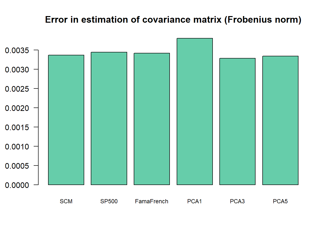

\[{\sf PRIAL} = 100\times \frac{\|\boldsymbol{\Sigma}_{\sf scm} - \boldsymbol{\Sigma}_{\sf true}\|_F^2 - \|\hat{\boldsymbol{\Sigma}} - \boldsymbol{\Sigma}_{\sf true}\|_F^2}{\|\boldsymbol{\Sigma}_{\sf scm} - \boldsymbol{\Sigma}_{\sf true}\|_F^2}\]

ref <- norm(Sigma_SCM - Sigma_true, "F")^2
PRIAL <- 100*(ref - error^2)/ref
print(PRIAL)
#>        SCM      SP500 FamaFrench       PCA1       PCA3       PCA5 
#>   0.000000  -4.698549  -3.071516 -27.761956   4.584330   1.335386
barplot(PRIAL, main = "PRIAL for estimation of covariance matrix", 
        col = "bisque3", cex.names = 0.75, las = 1)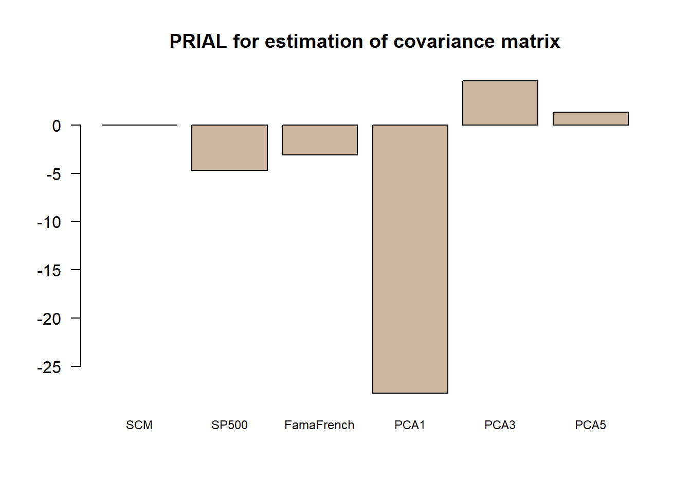

The final conclusion is that using factor models for covariance matrix estimation may help. In addition, it is not clear that using explicit factors helps as compared to the statistical factor modeling.

5.6 Edhec smart beta