Homework 3 ) Q3

library(ggplot2)

midwest

## # A tibble: 437 x 28
##      PID county state  area poptotal popdensity popwhite popblack popamerindian
##    <int> <chr>  <chr> <dbl>    <int>      <dbl>    <int>    <int>         <int>
##  1   561 ADAMS  IL    0.052    66090      1271.    63917     1702            98
##  2   562 ALEXA… IL    0.014    10626       759      7054     3496            19
##  3   563 BOND   IL    0.022    14991       681.    14477      429            35
##  4   564 BOONE  IL    0.017    30806      1812.    29344      127            46
##  5   565 BROWN  IL    0.018     5836       324.     5264      547            14
##  6   566 BUREAU IL    0.05     35688       714.    35157       50            65
##  7   567 CALHO… IL    0.017     5322       313.     5298        1             8
##  8   568 CARRO… IL    0.027    16805       622.    16519      111            30
##  9   569 CASS   IL    0.024    13437       560.    13384       16             8
## 10   570 CHAMP… IL    0.058   173025      2983.   146506    16559           331
## # … with 427 more rows, and 19 more variables: popasian <int>, popother <int>,
## #   percwhite <dbl>, percblack <dbl>, percamerindan <dbl>, percasian <dbl>,
## #   percother <dbl>, popadults <int>, perchsd <dbl>, percollege <dbl>,
## #   percprof <dbl>, poppovertyknown <int>, percpovertyknown <dbl>,
## #   percbelowpoverty <dbl>, percchildbelowpovert <dbl>, percadultpoverty <dbl>,
## #   percelderlypoverty <dbl>, inmetro <int>, category <chr>

options(scipen=999)

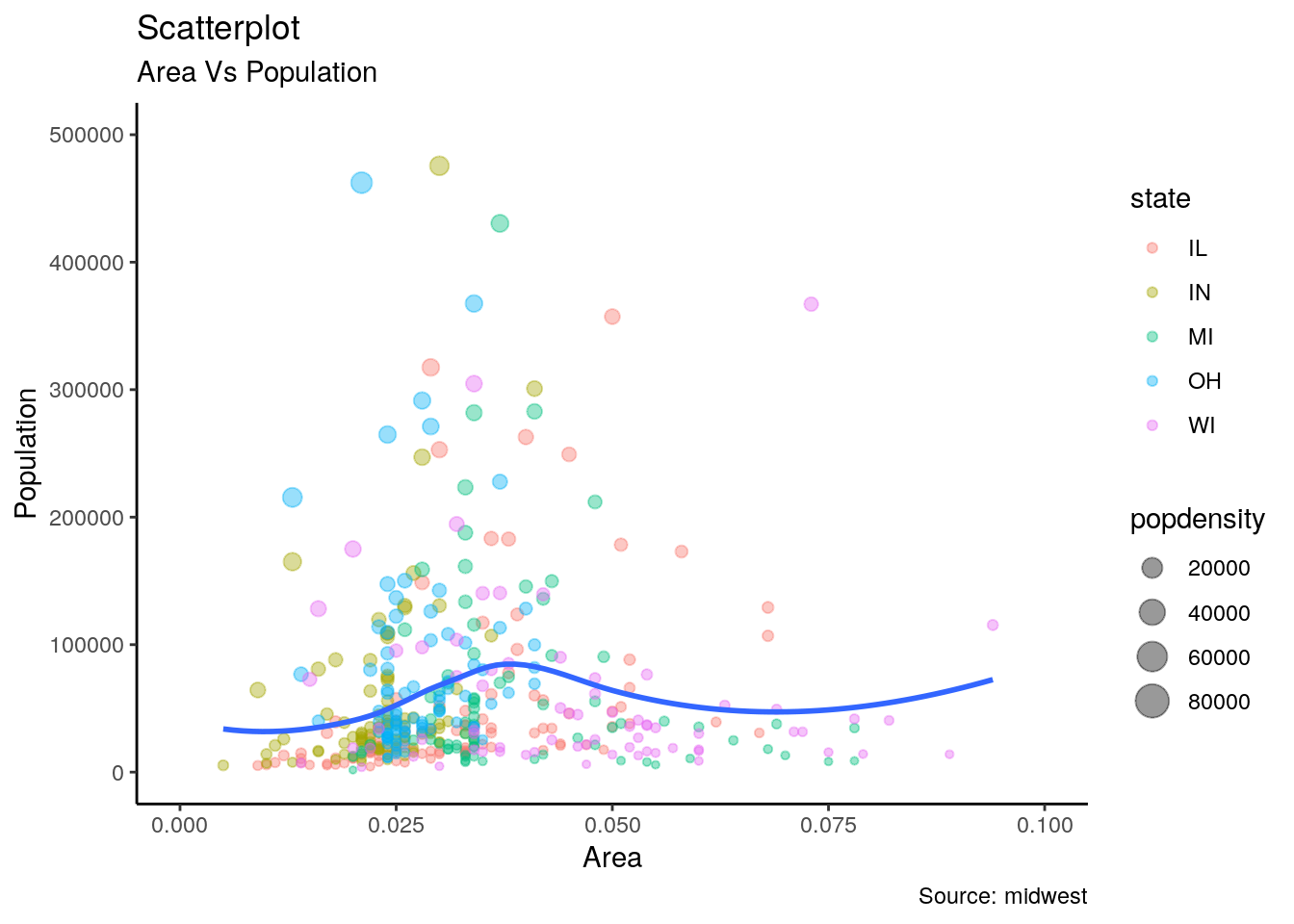
g3 <- ggplot(midwest, aes(area, poptotal,size=popdensity)) + geom_point(aes(color=state),alpha=0.4) + 
  xlim(0, 0.1) + 
  ylim(0, 500000) +
  theme_classic() + 
  labs(title="Scatterplot",subtitle = "Area Vs Population",x="Area",y="Population",caption = "Source: midwest")

3.1 Final Output

g3 +
  geom_smooth(se=F,show.legend=F)

## `geom_smooth()` using method = 'loess' and formula 'y ~ x'