Chapter 3 Generate sample GP

library(ggplot2)
library(dplyr)
library(tidyr)
library(reshape2)
library(RColorBrewer)
library(MASS)
library(ggsci)
library(kernlab)

D = 500
K = 5
V = 50
T = 100
G = 20
sigma_epsilon = 0.1  # Individual error term standard deviation

# Placeholder for GP Predictions and Original Densities
gppreds <- list()
gp_fits <- list()
original_densities <- list()

# Sample data
set.seed(42)  # For reproducibility
m = readRDS("samplediseasemerged.rds")
num_sample = K
samp = sample(1:nrow(m), num_sample)
sampled_topic = m$exclude_name[samp]

# Define a common grid for x values
common_grid <- seq(30, max(m$age_diag), length.out = 100)
sigmasq_noise = 0.01
# Fit Gaussian Processes for each topic
for (i in 1:length(sampled_topic)) {
  # Select data for the specific disease
  disease_data <- m[m$exclude_name %in% sampled_topic[i],]
  
  # Calculate density
  density_data <- density(disease_data$age_diag)
  
  # Fit Gaussian Process
  gp_fit <- gausspr(x = density_data$x, y = density_data$y, kernel = "rbfdot", kpar = "automatic")
  gp_fits[[i]] <- gp_fit
   # Store original density and predictions
  original_densities[[i]] <- data.frame(x = density_data$x, y = density_data$y, phenotype = sampled_topic[i])
  
  y_pred=predict(gp_fit, common_grid)
  gppreds[[i]] <- data.frame(x = common_grid, y = y_pred, phenotype = sampled_topic[i])
}

## Using automatic sigma estimation (sigest) for RBF or laplace kernel 
## Using automatic sigma estimation (sigest) for RBF or laplace kernel 
## Using automatic sigma estimation (sigest) for RBF or laplace kernel 
## Using automatic sigma estimation (sigest) for RBF or laplace kernel 
## Using automatic sigma estimation (sigest) for RBF or laplace kernel

# Combine all original densities and predictions into data frames
original_density_df <- do.call(rbind, original_densities)
gp_predictions <- do.call(rbind, gppreds)

# Plot using ggplot2
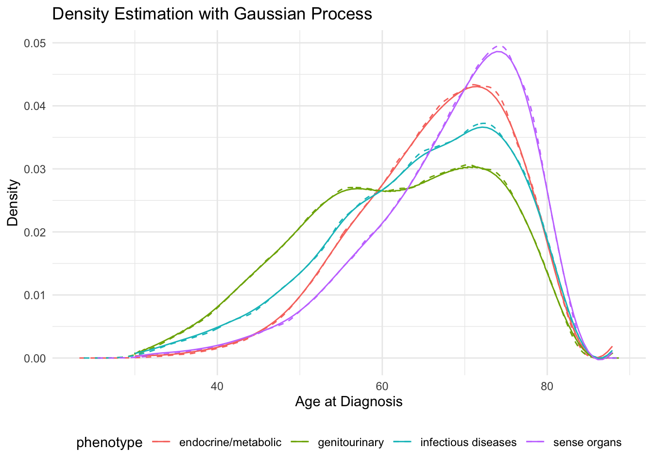
ggplot() +
  geom_line(data = original_density_df, aes(x = x, y = y, color = phenotype), linetype = "dashed") +
  geom_line(data = gp_predictions, aes(x = x, y = y, color = phenotype)) +
  labs(title = "Density Estimation with Gaussian Process",
       x = "Age at Diagnosis",
       y = "Density") +
  theme_minimal() +
  theme(legend.position = "bottom")

# Simulate individual-specific topic weights
genetic_scores <- array(runif(n = D * K * G, min = -1, max = 1), dim = c(D, K, G))
gamma <- matrix(runif(K * G, min = -0.5, max = 0.5), nrow = K, ncol = G)
gen_effect <- matrix(NA, nrow = D, ncol = K)

for (d in 1:D) {
  for (k in 1:K) {
    for (g in 1:G) {
      gen_effect[d, ] <- plogis(genetic_scores[d, , ] %*% gamma[k, ])
    }
  }
}

logit_func <- function(x) { log(x / (1 - x)) }

# Define the individual-level temporal covariance function (RBF Kernel)
# Define the individual-level temporal covariance function (RBF Kernel) with variance scaling
rbf_kernel <- function(x, y, length_scale = 10, variance = 0.01) {
  variance * exp(-0.5 * (x - y)^2 / length_scale^2)
}


# Generate the temporal covariance matrix for the individual-level deviations
time_points <- seq(1, T)
K_eta <- outer(time_points, time_points, rbf_kernel)

topic_weights <- array(NA, dim = c(D, K, T))
topic_weights_norm <- array(NA, dim = c(D, K, T))
topic_weights_pop <- array(NA, dim = c(K, T))
topic_weights_norm_pop <- array(NA, dim = c(K, T))

sigmasq_noise = 0.001
for (k in 1:K) {
  gp_fit <- gp_fits[[k]]
  gp_mean <- predict(gp_fit, common_grid)
  #K_xx <- kernelMatrix(gp_fit@kernelf, common_grid)
  # K_x <- kernelMatrix(gp_fit@kernelf, observed_data$x, common_grid)
  # K_inv <- solve(kernelMatrix(gp_fit@kernelf, observed_data$x) + diag(sigmasq_noise, length(observed_data$x)))
  # 
  # mu_post <- K_x %*% K_inv %*% observed_data$y
  # K_post <- K_xx - K_x %*% K_inv %*% t(K_x)
  # 
  # Ensure GP mean is within probability bounds
  gp_mean <- pmax(gp_mean, 1e-5)
  
  for (i in 1:D) {
    # Draw individual-level deviations from the posterior distribution
    K_eta=diag(sigmasq_noise,T)
    individual_deviation <- mvrnorm(n = 1, mu = rep(0, T), Sigma = K_eta)
    #genetic_adjustment <- gamma_k * gen_effect[i, k]
    
    # Draw individual-level topic weights from the posterior distribution
    #topic_weights[i, k, ] <- mvrnorm(n = 1, mu = mu_post + genetic_adjustment, Sigma = K_post)
    #topic_weights_norm[i, k, ] <- plogis(topic_weights[i, k, ])

    topic_weights_pop[k, ] = logit_func(gp_mean)
    ## same as simulating from eta where eta|data~GP(mu_gp+gamma*g,K_posterior)
    topic_weights[i, k, ] <- logit_func(gp_mean) + gen_effect[i, k] + individual_deviation
    topic_weights_norm[i, k, ] <- plogis(logit_func(gp_mean) + gen_effect[i, k] + individual_deviation)
    topic_weights_norm_pop[k, ] <- plogis(logit_func(gp_mean))
  }
}

# Generate topic activity
Topic_activity <- array(NA, dim = c(D, K, T))
for (d in 1:D) {
  for (k in 1:K) {
    Topic_activity[d, k, ] <- rbinom(n = T, prob = topic_weights_norm[d, k, ], size = 1)
  }
}

Theta_individual <- topic_weights_norm
Theta_pop <- topic_weights_norm_pop

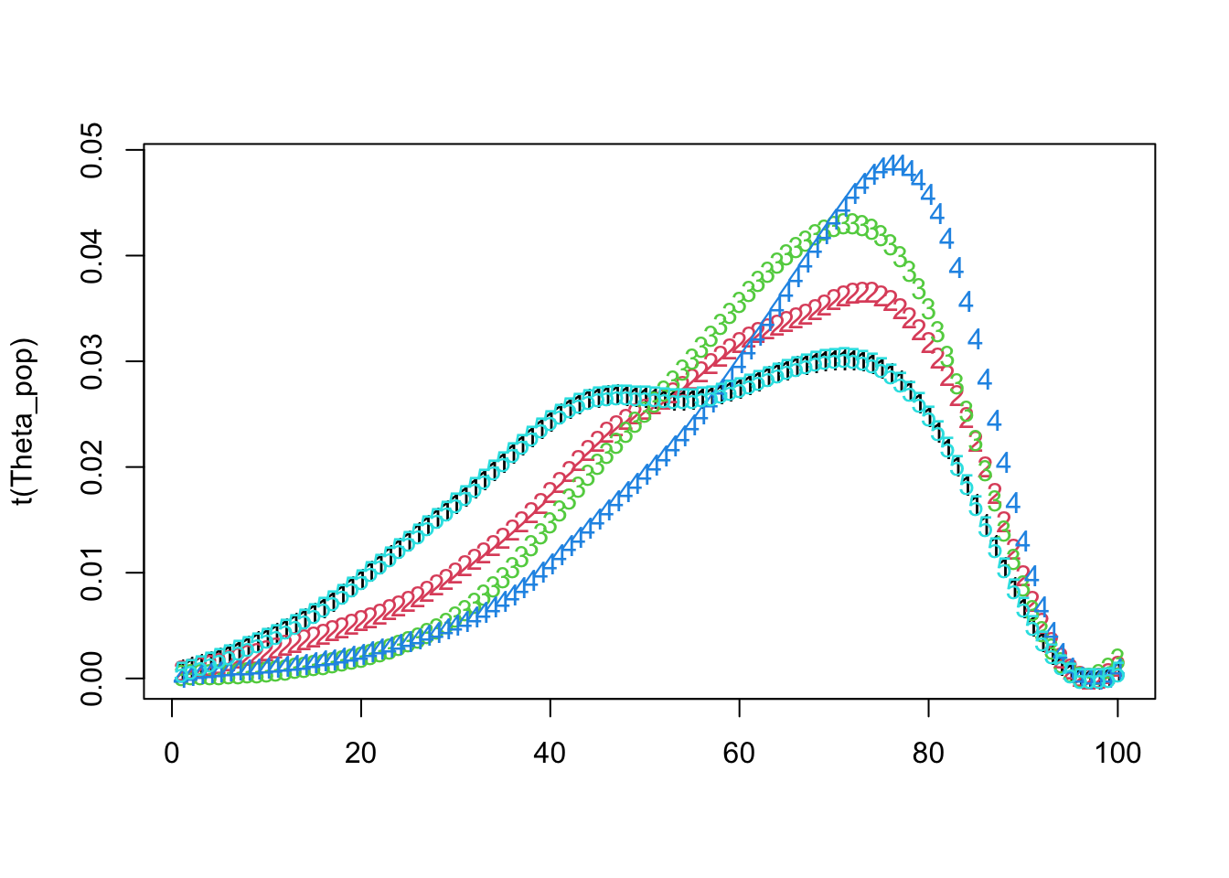
matplot(t(Theta_pop))

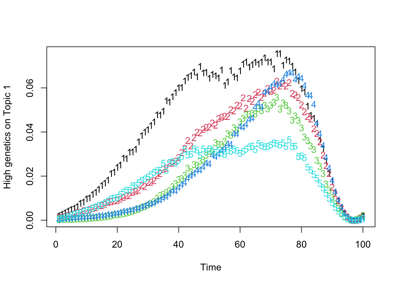
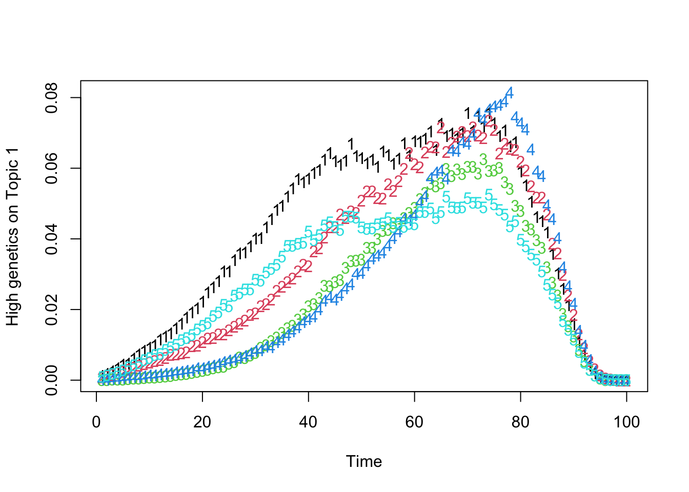
matplot(t(Theta_individual[which.max(gen_effect[, 1]), , ]), xlab = "Time", ylab = "High genetics on Topic 1")

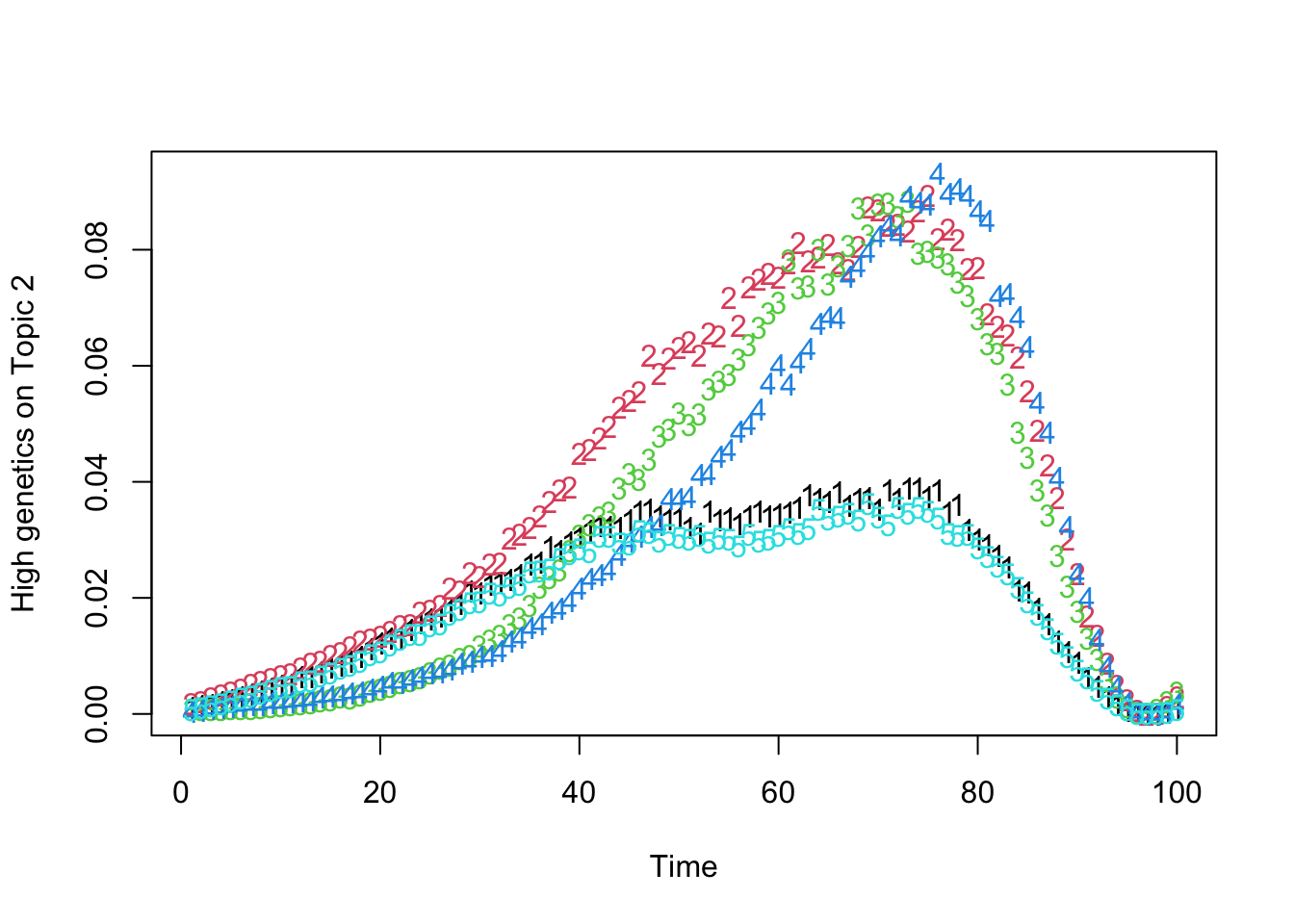
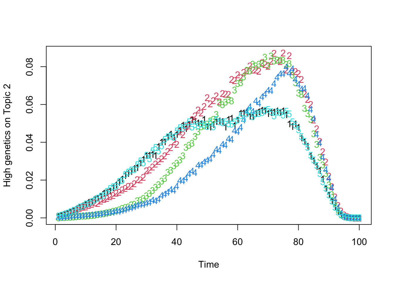
matplot(t(Theta_individual[which.max(gen_effect[, 2]), , ]), xlab = "Time", ylab = "High genetics on Topic 2")

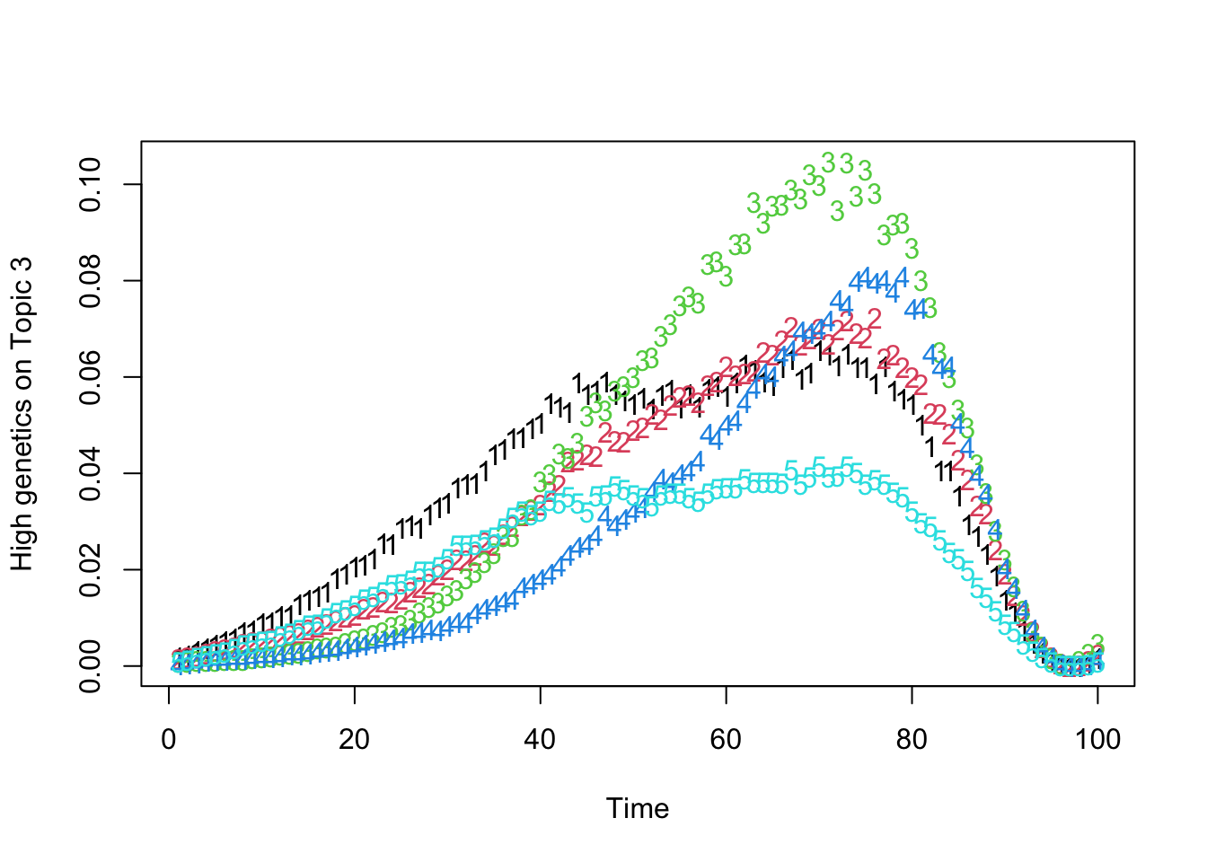
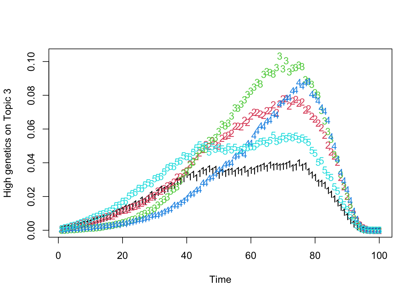
matplot(t(Theta_individual[which.max(gen_effect[, 3]), , ]), xlab = "Time", ylab = "High genetics on Topic 3")

D = 500
K = 5
V = 50
T = 100
G = 20

# Simulate individual-specific topic weights
genetic_scores <- array(runif(n = D * K * G, min = -1, max = 1), dim = c(D, K, G))
gamma <- matrix(runif(K * G, min = -0.5, max = 0.5), nrow = K, ncol = G)
gen_effect <- matrix(NA, nrow = D, ncol = K)


# Sample data
set.seed(42)  # For reproducibility
m = readRDS("samplediseasemerged.rds")
num_sample = K
samp = sample(1:nrow(m), num_sample)
sampled_topic = m$exclude_name[samp]

# Define a common grid for x values
common_grid <- seq(30, max(m$age_diag), length.out = 100)
sigmasq_noise <- 0.001

# Simulate individual-specific topic weights

for (d in 1:D) {
  for (k in 1:K) {
    for (g in 1:G) {
      gen_effect[d, ] <- plogis(genetic_scores[d, , ] %*% gamma[k, ])
    }
  }
}


# Placeholder for Gaussian Process fits and topic weights
gp_fits <- list()
topic_weights <- array(0, dim = c(D, K, T))
topic_weights_norm <- array(0, dim = c(D, K, T))

for (k in 1:K) {
  # Simulate some density data for fitting GP (replace this with your actual data)
  disease_data <- m[m$exclude_name %in% sampled_topic[k],]
  
  # Calculate density
  density_data <- density(disease_data$age_diag)
  
  # Fit Gaussian Process
  gp_fit <- gausspr(x = density_data$x, y = density_data$y, kernel = "rbfdot", kpar = "automatic")
  gp_fits[[k]] <- gp_fit
  
  # Extract kernel matrices
  K_train_train <- kernelMatrix(gp_fit@kernelf, density_data$x)
  K_train_common <- kernelMatrix(gp_fit@kernelf, density_data$x, common_grid)
  K_common_common <- kernelMatrix(gp_fit@kernelf, common_grid)
  
  # Noise variance
  sigma2_noise <- diag(sigmasq_noise, length(density_data$x))
  
  # Inverse of the noisy kernel matrix
  K_inv <- solve(K_train_train + sigma2_noise)
  
  # Posterior mean and covariance
  mu_post <- t(K_train_common) %*% K_inv %*% density_data$y
  K_post <- K_common_common - t(K_train_common) %*% K_inv %*% K_train_common
  
  # Ensure GP mean is within probability bounds
  mu_post <- pmax(mu_post, 1e-5)
  
  for (i in 1:D) {
    # Adjust posterior mean with genetic effects
    mu_post_adjusted <- logit_func(mu_post) + gen_effect[i, k]
    
    # Draw individual-level deviations from posterior covariance
    individual_deviation <- mvrnorm(n = 1, mu = rep(0, T), Sigma = K_post)
    
    # Combine to get the individual-level topic weights
    topic_weights_pop[k, ] = logit_func(mu_post)
    ## same as simulating from eta where eta|data~GP(mu_gp+gamma*g,K_posterior)

    topic_weights[i, k, ] <- mu_post_adjusted + individual_deviation
    topic_weights_norm[i, k, ] <- plogis(topic_weights[i, k, ])
  }
}

## Using automatic sigma estimation (sigest) for RBF or laplace kernel 
## Using automatic sigma estimation (sigest) for RBF or laplace kernel 
## Using automatic sigma estimation (sigest) for RBF or laplace kernel 
## Using automatic sigma estimation (sigest) for RBF or laplace kernel 
## Using automatic sigma estimation (sigest) for RBF or laplace kernel

Theta_individual <- topic_weights_norm
Theta_pop <- topic_weights_norm_pop

matplot(t(Theta_pop))

matplot(t(Theta_individual[which.max(gen_effect[, 1]), , ]), xlab = "Time", ylab = "High genetics on Topic 1")

matplot(t(Theta_individual[which.max(gen_effect[, 2]), , ]), xlab = "Time", ylab = "High genetics on Topic 2")

matplot(t(Theta_individual[which.max(gen_effect[, 3]), , ]), xlab = "Time", ylab = "High genetics on Topic 3")

Now plot acitivty:



``` r
melt_topic_activity <- function(activity_array) {
  activity_df <- melt(activity_array)
  names(activity_df) <- c("Individual", "Topic", "Time", "Activity")
  activity_df$Active <- ifelse(activity_df$Activity == 1, paste("Active", activity_df$Topic), "Inactive")
  return(activity_df)
}

df <- melt_topic_activity(Topic_activity)

# Define color palette
num_active_levels <- length(setdiff(unique(df$Active), "Inactive"))
softer_palette <- brewer.pal(min(num_active_levels, 8), "Set2")  # Use Set2 palette for up to 8 different active levels
active_levels <- setdiff(unique(df$Active), "Inactive")
colors_for_active <- setNames(softer_palette[1:num_active_levels], active_levels)
colors <- c("Inactive" = "white", colors_for_active)


# Plotting functions
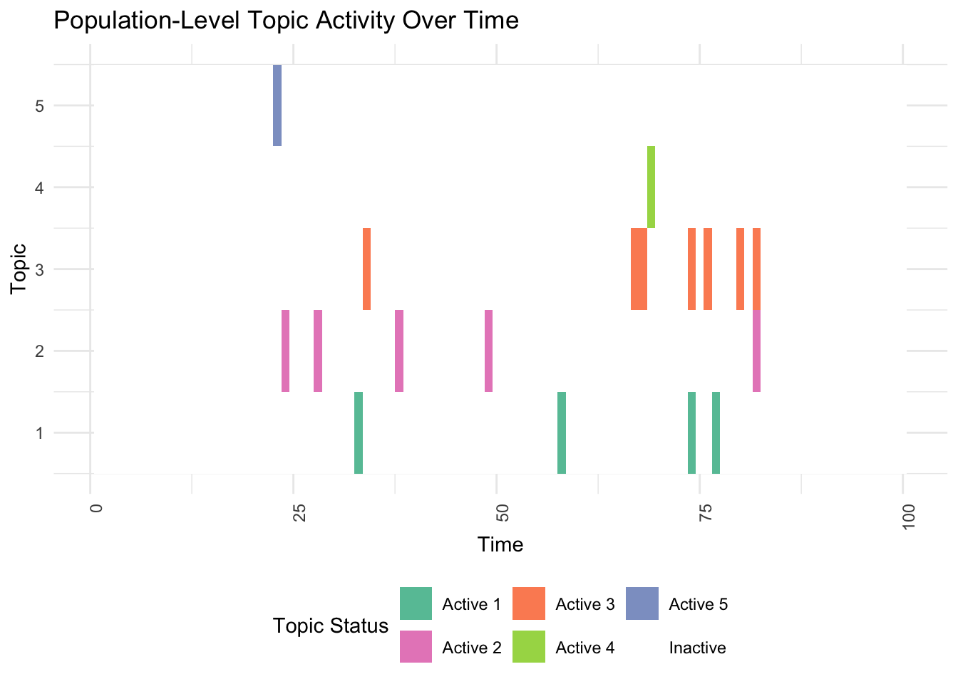
plot_population <- function(df) {
  ggplot(df, aes(x = Time, y = Topic, fill = Active)) +
    geom_tile() +
    scale_fill_manual(values = colors) +
    labs(title = "Population-Level Topic Activity Over Time",
         x = "Time", y = "Topic", fill = "Topic Status") +
    theme_minimal() +
    theme(axis.text.x = element_text(angle = 90, hjust = 1),
          legend.position = "bottom")
}

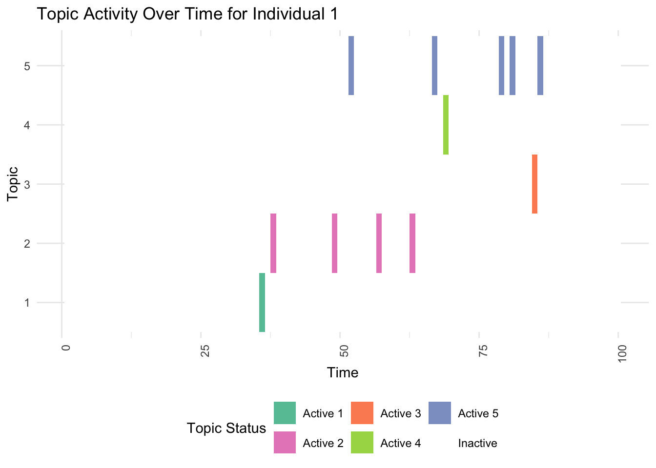
plot_individual <- function(df, individual_id) {
  individual_df <- df %>% filter(Individual == individual_id)
  ggplot(individual_df, aes(x = Time, y = as.factor(Topic), fill = Active)) +
    geom_tile() +
    scale_fill_manual(values = colors) +
    labs(title = paste("Topic Activity Over Time for Individual", individual_id),
         x = "Time", y = "Topic", fill = "Topic Status") +
    theme_minimal() +
    theme(axis.text.x = element_text(angle = 90, hjust = 1),
          legend.position = "bottom")
}

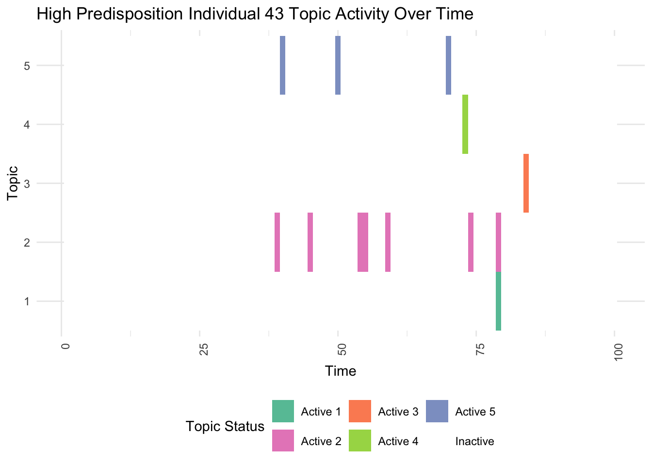
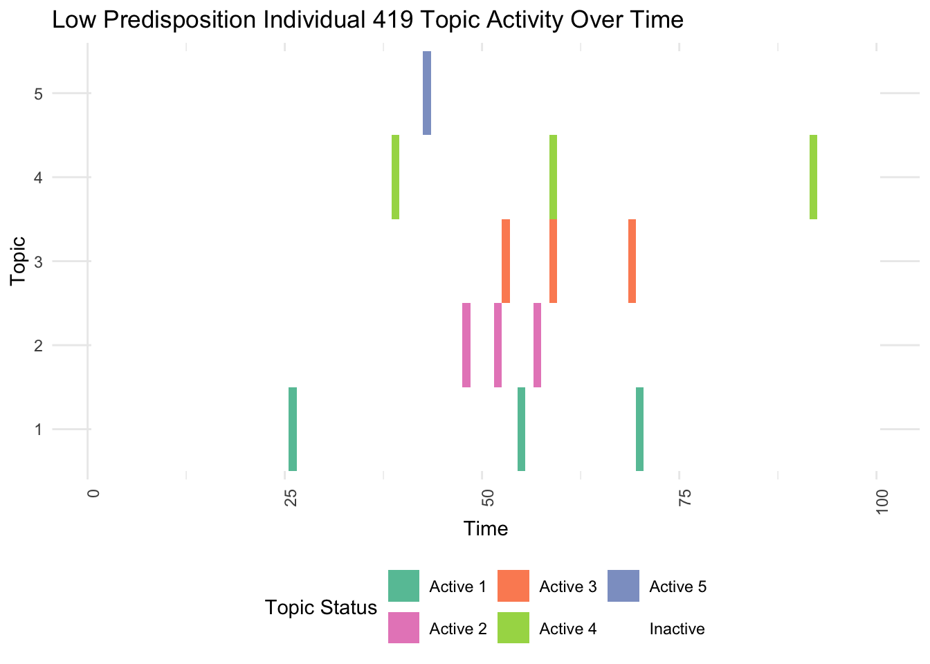
plot_high_predisposition <- function(df, individual_id) {
  high_predisposition_df <- df %>% filter(Individual == individual_id)
  ggplot(high_predisposition_df, aes(x = Time, y = as.factor(Topic), fill = Active)) +
    geom_tile() +
    scale_fill_manual(values = colors) +
    labs(title = paste("High Predisposition Individual", individual_id, "Topic Activity Over Time"),
         x = "Time", y = "Topic", fill = "Topic Status") +
    theme_minimal() +
    theme(axis.text.x = element_text(angle = 90, hjust = 1),
          legend.position = "bottom")
}


plot_low_predisposition <- function(df, individual_id) {
  high_predisposition_df <- df %>% filter(Individual == individual_id)
  ggplot(high_predisposition_df, aes(x = Time, y = as.factor(Topic), fill = Active)) +
    geom_tile() +
    scale_fill_manual(values = colors) +
    labs(title = paste("Low Predisposition Individual", individual_id, "Topic Activity Over Time"),
         x = "Time", y = "Topic", fill = "Topic Status") +
    theme_minimal() +
    theme(axis.text.x = element_text(angle = 90, hjust = 1),
          legend.position = "bottom")
}


# Identify individuals with high and low genetic predispositions
high_predisposition_individual <- which.max(rowSums(gen_effect))
low_predisposition_individual <- which.min(rowSums(gen_effect))

# 1. Population-Level Topic Activity
print(plot_population(df))

# 2. Individual-Level Topic Activity Across All Topics
print(plot_individual(df, 1))

# 3. Detailed View for an Individual with High Predispositions
print(plot_high_predisposition(df, high_predisposition_individual))

# 4. Detailed View for an Individual with Low Predispositions
print(plot_low_predisposition(df, low_predisposition_individual))

3.1 Plot theta

mf=melt(Theta_individual)
colnames(mf)=c("Individual","Topic","Time","Value")
ggplot(mf[mf$Individual%in%sample(D,1),],aes(x=Time,y=Value,group=as.factor(Topic),fill=as.factor(Topic)))+geom_area()+theme_classic()+labs(y="Theta",x="Age")+scale_fill_nejm()

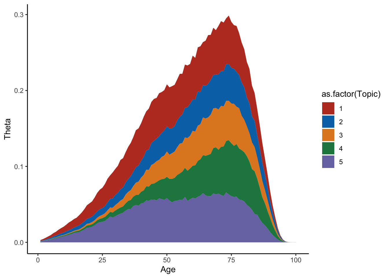
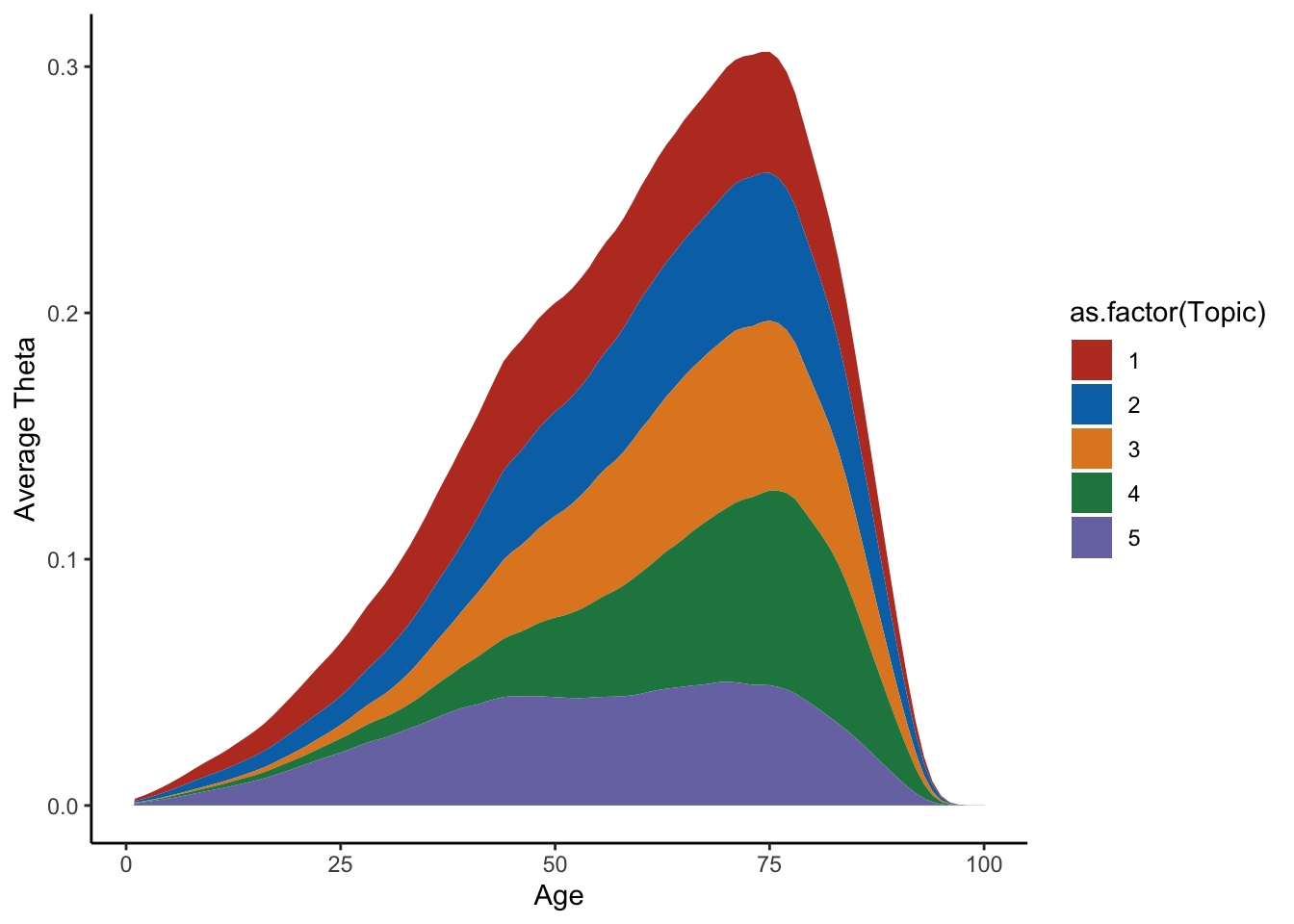
average=apply(Theta_individual,c(2,3),mean)
m=melt(average)
colnames(m)=c("Topic","Time","Value")
ggplot(m,aes(x=Time,y=Value,group=Topic,fill=as.factor(Topic)))+geom_area()+theme_classic()+labs(y="Average Theta",x="Age")+scale_fill_nejm()