7 Graph Analysis
knitr::include_graphics("images/grafo.png")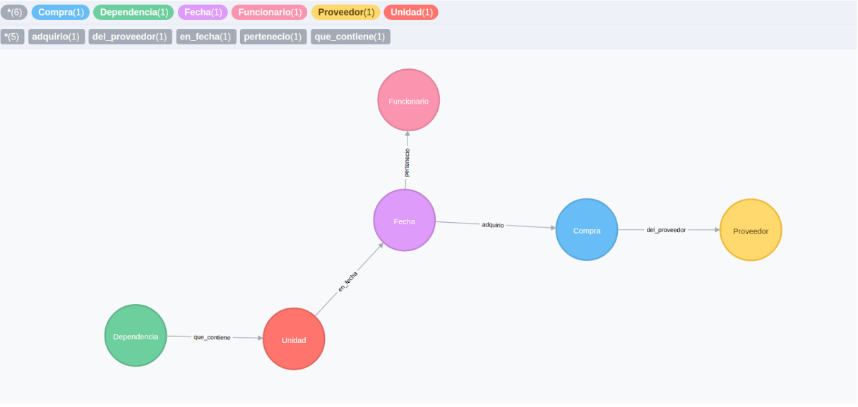
7.1 Suspicious Connections
Our data modeling process implies creating a fairly complex multi layered graph, for which not all centrality measures can be computed. We combined graph structure measures with more intuitive variables to include in our analysis:
7.1.1 Weighted degree centrality of bureaucrat \(i\), firm \(j\) or RU \(u\)
Weighted degree centrality of some vertex \(v\) is defined as follows:
\[C_{D}(v) := deg(v)\]
knitr::include_graphics("images/centralidad.png")7.1.2 Concentration of bureaucrat connections
Inspired in the construction of Hirschman Herfindahl Index (HHI), this variable is constructed as:
\[H_i = \sum_j w_{i,j}^2\]
where \(w_{i,j}\) is weight of firm \(j\) in the total value assigned through contracts by bureaucrat \(i\).
knitr::include_graphics("images/concentracion.png")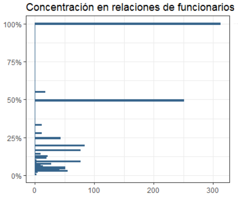
7.1.3 Concentration of firm connections
This is intuitively seen as some probability that firm \(j\) has at least one crony relationship.
\[\bar{w_k} = \underset{i}{\text{max } w_{i,k}}\]
7.1.4 Distance to other agents
We also computed the shortest paths distance to a sanctioned firm, to a ghost firm or to a bureaucrat using Dijkstra’s algorithm. The shortest path distance calculates the number of nodes that must be visited when connecting two specific nodes, adding a unit to the distance for each node visited. It does this for all possible paths between two nodes and then selects the minimum distance.
In general, Dijkstra’s algorithm assigns some initial distance values and will try to improve them step by step as explained below:
- Assign to every node an initial distance value.
- Sets the initial node as the current node and marks all other nodes unvisited.
- Creates a set of all the unvisited nodes, called the unvisited set.
- For the current node, it considers all of its neighbors and calculates their tentative distances. It then compares the newly calculated tentative distance to the current assigned value and assigns the smaller one. Otherwise, it keeps the current value.
- When all of the neighbors of the current node have been considered, it marks the current node as visited and removes it from the unvisited set. A visited node will never be checked again.
- The algorithm reaches an end when either the destination node is no longer in the unvisited set or when the distance among the unvisited nodes is infinity (i.e. there is no connection between the nodes).
- If the algorithm does not reach an end, it selects the unvisited node that is marked with the smallest tentative distance, sets it as the new “current node”, and goes back to step 4
In later steps we will use the shortest path to identify centrality meassures in the graph.