2 K-Means clustering
2.1 Introduction: kNN versus K-Means
In the kNN method we started from a known grouping of objects, with the challenge of using characteristics as predictors of group membership.
We predict a person’s membership from the majority group membership of his or her neigbours.
We were able to train the model because we already have data about the grouping (for example: rejected and accepted loan requests).
But in some cases, the challenge is to find groups of objects that are similar in terms of a number of selected criteria.
The difference with the kNN method is that we do not know in advance which groups there are, or how many.
Another difference is that we are particularly interested in the profiles of these groups.
With the kNN method, the emphasis was on the correct classification but we were not primarily concerned about the group profiles: we didn’t actually spend a word on how people whose loans were accepted or rejected, differ in terms of age, gender, experience, skills, and so on.
2.2 The Algorithm
The approach in K-means clustering has a lot in common with the kNN method, but still it is fundamentally different.
The letter k has different meanings in the two methods (kNN and K-means).
- In the kNN method the k stands for the number of nearest neighbours to which the object to be classified is compared.
- In K-means, k signifies the number of clusters (groups) that we want to form.
In both methods, the concept of distance comes in.
In K-means, objects are assigned to a cluster based on the Euclidean distance between the object and the center of the cluster, also referred to as the cluster centroid.
But we do not know in advance how many clusters there are, and we do not know what the clusters will look like.
That is why we work in two steps.
- First, we determine the optimal number of clusters, and then
- We determine starting values for each cluster.
2.3 Determining the Number of Clusters
The number of clusters can be determined in three ways.
- The first way is a rule of thumb that sets the number of clusters to the square root of half the number of objects.
If we want to cluster 200 objects, the number of clusters would be √(200/2)=10.
We then have a relatively large number of clusters (10) compared to the average size of the clusters (20 objects per cluster).
The rule of thumb works well when cluster analysis is applied to relatively small files.
In the era of big data with files of thousands of objects (transactions, people, messages), the number of clusters would increase dramatically. With, say, 2 million objects, the number of groups would be 1,000 - which is not exactly a compact way to structure information.
- A better method - but not always possible - is to determine the number of clusters using similar classifications in use.
Examples:
- For the intensity of use of a product or service, marketing theory uses a three-way division in light, medium and heavy users.
- In tourism, research institute Motivaction uses a division into 5 categories (traditionals; mainstreamers; upperclass quality seekers; postmoderns and achievers).
If we do dispose of any existing classifications beforehand, we can statistically underpin the number of clusters.
- A statistical measure for homogeneity
The purpose of cluster analysis is to form groups of objects …
- which resemble one other as closely as possible, and
- which differ as much as possible from objects in the other clusters.
In other words, we are interested in the homogeneity of clusters.
Homogeneity can be determined by the variation of the characteristics of the objects within the cluster: the less variation, the more homogeneous the cluster is.
As a rule: variation decreases as the clusters get smaller.
In the extreme case, a single object forms its own little cluster, and variation is reduced to 0. But then, unfortunately, we have made no progress at all! We now have as many clusters as we had objects.
We do accept a certain level of variation within clusters, as long as the clusters are interpretable and deviate from other clusters.
A statistical measure of the variation is the so-called within group sum of squares (wss).
We can plot the wss against the number of clusters.
Often, we see a kink (the “elbow”) in the curve: the wss first drops quickly but then evens out. At the elbow, the optimal number of clusters has been reached. Adding more (and therefore smaller) clusters hardly leads to more homogeneous clusters, and often to the splitting off of small clusters that are hardly interesting.
Quick-R explains how to produce the curve.
Let’s apply it to an example.
A travel agency offers a variety of trips, including trips based on the principles of sustainable tourism.
To find out what is important to tourists, a short survey was used from which scores are derived for the importance of six characteristics:
- Willingness to pay (wtp) more for sustainable tourism
- The preceived importance of sustainable tourism (rt)
- Price sensitivity (price)
- Quality of accommodation (accom)
- Quality of services (serv)
- The importance of nature and scenery (geo).
The data of 200 respondents are in a file created in STATA.
In addition to the 6 scores, we also have information about:
- Gender (male, a 0/1 dummy variable, 0=woman, 1=male)
- Age (age, young/middle/old)
- Income (income, low/medium/high), and
- Region (dummy variables for tourists from the EU [eu] and from USA [us]).
The lines below read the data and give the structure with the str() command.
Check for yourself with the summary() command that all values are in the expected range. It seems there are also no missing values.
library(foreign)
tourist <- read.dta("tourist.dta",convert.factors=FALSE)
str(tourist)
## 'data.frame': 200 obs. of 11 variables:
## $ male : num 1 0 1 1 0 0 0 0 0 0 ...
## $ age : int 2 2 2 2 3 1 3 1 3 3 ...
## $ income: num 2 1 2 1 2 2 1 2 1 2 ...
## $ eu : num 1 0 1 1 0 1 0 0 1 0 ...
## $ us : num 0 1 0 0 1 0 0 0 0 1 ...
## $ wtp : num 3 2 2 2 2 3 2 3 5 2 ...
## $ price : num 4 3.5 3 2 3.5 3 1 4.5 3 3 ...
## $ accom : num 2.5 5 4.5 5 4.5 4 5 4 3.5 4 ...
## $ serv : num 3 4 4 2 3 4 5 4 3 4 ...
## $ rt : num 4.6 4.6 4.6 3.6 4.4 ...
## $ geo : num 5 5 5 5 5 5 5 5 5 4 ...
## - attr(*, "datalabel")= chr " "
## - attr(*, "time.stamp")= chr "19 Apr 2016 12:34"
## - attr(*, "formats")= chr [1:11] "%9.0g" "%9.0g" "%9.0g" "%9.0g" ...
## - attr(*, "types")= int [1:11] 254 251 254 254 254 254 254 254 254 254 ...
## - attr(*, "val.labels")= chr [1:11] "" "age" "" "" ...
## - attr(*, "var.labels")= chr [1:11] "Male (dummy)" "age" "inkomen" "EU resident" ...
## - attr(*, "version")= int 12
## - attr(*, "label.table")=List of 1
## ..$ age: Named int [1:3] 1 2 3
## .. ..- attr(*, "names")= chr [1:3] "<35" "35-55" "56+"summary(tourist)## male age income eu us
## Min. :0.000 Min. :1.00 Min. :1.00 Min. :0.000 Min. :0.00
## 1st Qu.:0.000 1st Qu.:1.00 1st Qu.:2.00 1st Qu.:0.000 1st Qu.:0.00
## Median :1.000 Median :2.00 Median :2.00 Median :1.000 Median :0.00
## Mean :0.565 Mean :2.01 Mean :2.01 Mean :0.625 Mean :0.22
## 3rd Qu.:1.000 3rd Qu.:3.00 3rd Qu.:2.00 3rd Qu.:1.000 3rd Qu.:0.00
## Max. :1.000 Max. :3.00 Max. :3.00 Max. :1.000 Max. :1.00
## wtp price accom serv rt
## Min. :1.000 Min. :1.000 Min. :2.00 Min. :1.000 Min. :1.800
## 1st Qu.:2.000 1st Qu.:3.000 1st Qu.:4.00 1st Qu.:3.000 1st Qu.:3.800
## Median :3.000 Median :3.500 Median :4.00 Median :4.000 Median :4.200
## Mean :2.915 Mean :3.333 Mean :4.21 Mean :3.737 Mean :4.144
## 3rd Qu.:4.000 3rd Qu.:4.000 3rd Qu.:5.00 3rd Qu.:4.000 3rd Qu.:4.600
## Max. :5.000 Max. :5.000 Max. :5.00 Max. :5.000 Max. :5.000
## geo
## Min. :2.00
## 1st Qu.:5.00
## Median :5.00
## Mean :4.78
## 3rd Qu.:5.00
## Max. :5.00Our goal is to cluster the tourists according to what they consider important, as indicated in the last 6 variables in the data frame (columns 6 to 11, in the data frame tourist).
We create a data frame with just these 6 characteristics. Then we plot the wss against the number of clusters.
touristImportance <- tourist[,6:11]
k <- 12 # Max number of cluster for wss-plot
wss <- (nrow(touristImportance)-1)*sum(apply(touristImportance,2,var)); wss[1]
## [1] 832.8022for (i in 2:k) wss[i] <- sum(kmeans(touristImportance, centers=i)$withinss)
plot(1:k, wss, type="b", xlab="# Clusters", ylab="Heterogeneity")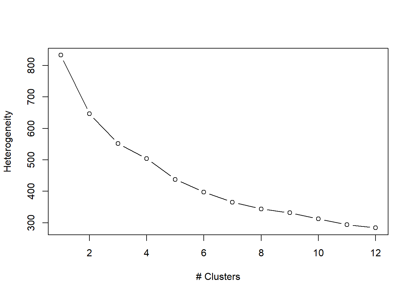
The plot shows that, indeed, the heterogeneity of the clusters decreases with the number of clusters. It has to.
The decrease, however, is leveling off: the decrease is strongest when we go from 1 to 2 clusters. The decline is slightly less pronounced from 2 to 3; and so on.
There is not a very clear elbow in the curve in this case.
The heterogeneity at 5 clusters is half of the base situation, and the gain from moving up to 12 clusters is small (from approximately 400 to 300). Five clusters seems like a good choice. But normally we experiment: are the results easier to interpret with 4 or 6 clusters?
Remember: cluster analysis is an exploratory method: we simply do not know the number and nature of clusters in advance!
We also call this unsupervised learning, in Machine Learning jargon.
The K-Means method generates new data (clusters) that must be named by the analyst.
The value of the analysis lies in the interpretation.
The results cannot be applied to a test set!
Experimentation is all the more important as K-means has different algorithms for determining clusters.
An iterative method is to first randomly select k objects as the initial clusters, and then assign other objects to the cluster, after which the center (centroid) of the cluster is re-determined.
The procedure ends when no more objects change clusters.
The result of K-means is sensitive to the random selection of objects for the initial solution, and it is therefore recommended to repeat the procedure with different starting points, to see how robust the solution is.
2.4 Standardize or Normalize
As in the k-NN method, the characteristics used for clustering must be measured in comparable units.
In this case, units are not an issue since all 6 characteristics are expressed on a 5-point scale. Normalization or standardization is not necessary.
2.5 The Analysis
2.5.1 Step 1: Preparing the Data
We have already gone through step 1. That is, we have read the data.
It concerns 200 tourists and their data on age, gender, income and nationality, and their opinion on the importance of six characteristics of tourist destinations and places to stay.
Because we only want to cluster the tourists on the 6 characteristics, we have created a file with only those variables.
We have already argued that normalizing or standardizing the data is not necessary.
Incidentally, it doesn’t hurt to do so, and many researchers always standardize the data, with the reason that the cluster centers are easier to interpret.
2.5.2 Step 2: Training the Model
The K-means method is unsupervised learning, in which clustering results in new data.
There is no test set to evaluate if membership of a still to be formed cluster is correctly predicted!
However, we will evaluate the model on the basis of other characteristics in the data set.
The question is, does clustering help us? We can check whether the clusters also differ in terms of background characteristics (such as age and nationality) that make it possible, in marketing terms, to approach the segments (clusters) with a differentiated marketing strategy.
We train the model with functions from the package stats. Like the foreign package, this package is part of the system library and, hence, does not need to be installed separately. But it must be invoked with the library() command.
The function from the stats package is kmeans().
In brackets we put the name of the data set and the number of clusters.
We store the results in an object that contains all the information we need - as we will see.
One of the characteristics is the size of the clusters (the number of tourists in each cluster).
The size of the clusters is a vector (size) in the cluster object.
The size of the clusters varies from 26 (cluster 3) to 68 (cluster 5).
To generate the same results, use the set.seed() command. Not using this command or changing the start number will give a slightly different outcome: the outcome is sensitive to the start set!
Therefore, test the robustness of the analysis by repeating with other starting values.
For reassurance, it is rare for repetition to produce substantially different results, especially if the variables do not show any outliers.
With a 5-point scale it is not possible to have outliers anyway, as the scale is restricted to values in the range of 1 to 5. But, still, for the same reasons, it is crucially important to check the data for errors: a coding error (a record with a value of 55, on a scale of 1-5) will affect the outcome.
library(stats)
set.seed(35753)
touristCluster <- kmeans(touristImportance, 5)
touristCluster$size
## [1] 33 68 26 38 35It is equally interesting to look at what exactly the five clusters represent.
The most insightful way is to make an overview of the cluster centers (centroids).
This information is in the same object (touristCluster), in the matrix centers.
We can print this information directly into the console:
round(touristCluster$centers, 2)## wtp price accom serv rt geo
## 1 3.70 4.17 4.73 4.35 4.64 4.91
## 2 2.03 3.79 4.25 3.88 4.09 4.78
## 3 2.38 2.83 3.31 2.40 4.17 4.77
## 4 2.71 2.07 4.57 4.33 3.95 4.79
## 5 4.51 3.40 3.93 3.24 3.98 4.66Each row represents a cluster.
- The first cluster has high mean scores on all variables.
- The second cluster scores low on the WTP (willingness to pay extra), and on the importance of the price of the trip. Scores on quality of accommodation and services, on the other hand, are higher than in the other clusters.
- For all clusters we see that the scores on geo are high (4.67 or higher, on a 5-point scale). This aspect is therefore hardly distinctive and can possibly be omitted in a subsequent run.
2.5.3 Step 3: Evaluating the Model
Since we are exploring and searching for hidden homogeneous groups of tourists, we cannot use a test set to check whether the model predicts correctly. There is nothing to predict!
The evaluation is based on the answers to three questions:
- Are the clusters large enough to be of any use (substance)?
- Are there clear, interpretable differences between the clusters, or can we label them in a meaningful way?
- Do the clusters provide information that gives rise to specific actions (actionable)?
The last question is important. If we can’t do anything with the information, then the results are interesting, or nice to know, but not useful.
For the interpretation, we draw up a profile of the clusters.
Now that we know that there are clusters with different motives and behavioral characteristics, we can determine who are the cluster members. Are they old or young tourists? Rich or Poor? Europeans or Americans?
To make the profiles, we can extract a vector from the touristCluster object that contains, for all tourists, the cluster in which they have been classified.
We can add this vector to the original file in which we also have information about age, gender, income and nationality.
In the second line we ask R for the first 6 tourists in the file to print the information about cluster, age, income, and nationality.
tourist$cluster <- touristCluster$cluster
tourist[1:6, c("cluster","age","income","eu","us")]
## cluster age income eu us
## 1 3 2 2 1 0
## 2 2 2 1 0 1
## 3 2 2 2 1 0
## 4 3 2 1 1 0
## 5 2 3 2 0 1
## 6 4 1 2 1 0For an overall picture, we can use the aggregate() function that provides statistical information (for example, the mean age, or the mean nationality) for each cluster.
Of course mean nationality is a weird concept. But since we have made use of dummy variables, the mean just indicates the proportion of tourists with that specific characteristic.
aggregate(data=tourist, age ~ cluster, mean)## cluster age
## 1 1 1.909091
## 2 2 1.926471
## 3 3 1.961538
## 4 4 2.157895
## 5 5 2.142857aggregate(data=tourist, eu ~ cluster, mean)## cluster eu
## 1 1 0.5757576
## 2 2 0.6617647
## 3 3 0.6923077
## 4 4 0.5526316
## 5 5 0.6285714aggregate(data=tourist, us ~ cluster, mean)## cluster us
## 1 1 0.2424242
## 2 2 0.2352941
## 3 3 0.1538462
## 4 4 0.2368421
## 5 5 0.2000000aggregate(data=tourist, income ~ cluster, mean)## cluster income
## 1 1 2.090909
## 2 2 1.970588
## 3 3 1.961538
## 4 4 2.131579
## 5 5 1.914286aggregate(data=tourist, male ~ cluster, mean)## cluster male
## 1 1 0.5757576
## 2 2 0.6323529
## 3 3 0.5769231
## 4 4 0.5526316
## 5 5 0.42857142.6 Putting It All Together
We can, literally, put it all together by combining the relevant information in a data frame, and then export the data frame to Excel or another tool, to further analyze and summarize the information, and prepare it for presentation.
outlook <- round(touristCluster$centers, 2)

tourist$cluster <- touristCluster$cluster
tourist[1:6, c("cluster","age","income","eu","us")]
## cluster age income eu us
## 1 3 2 2 1 0
## 2 2 2 1 0 1
## 3 2 2 2 1 0
## 4 3 2 1 1 0
## 5 2 3 2 0 1
## 6 4 1 2 1 0t1 <- aggregate(data=tourist, age ~ cluster, mean)
t2 <- aggregate(data=tourist, eu ~ cluster, mean)
t3 <- aggregate(data=tourist, us ~ cluster, mean)
t4 <- aggregate(data=tourist, income ~ cluster, mean)
t5 <- aggregate(data=tourist, male ~ cluster, mean)
t <- cbind(t1,t2$eu,t3$us,t4$income,t5$male, outlook)
round(t,2)## cluster age t2$eu t3$us t4$income t5$male wtp price accom serv rt geo
## 1 1 1.91 0.58 0.24 2.09 0.58 3.70 4.17 4.73 4.35 4.64 4.91
## 2 2 1.93 0.66 0.24 1.97 0.63 2.03 3.79 4.25 3.88 4.09 4.78
## 3 3 1.96 0.69 0.15 1.96 0.58 2.38 2.83 3.31 2.40 4.17 4.77
## 4 4 2.16 0.55 0.24 2.13 0.55 2.71 2.07 4.57 4.33 3.95 4.79
## 5 5 2.14 0.63 0.20 1.91 0.43 4.51 3.40 3.93 3.24 3.98 4.66# install.packages("writexl")
# library(writexl)
# write_xlsx(t,"t.xlsx")In Excel, we have colored the particularly high and low scores - in green and red respctively, on all the variables used in clustering the objects.
The profiles in the first columns are marked yellow, if certain background characteristics stand out from the other clusters.

Some tentative conslusions:
- Cluster 1 consists of mainly young male tourists, who are willing to pay extra for responsibly managed sites. They do value responsible tourism.
- Cluster 2 has a similar demographic outlook, but here, the male youngsters are not willing to pay extra for responsibly managed sites.
- Cluster 3 consists of many European tourists, who are not willing to pay extra. Strikingly, their interest in high quality accomodation and services is lower than for the other clusters.
- Cluster 4 looks like a traditional, somewhat older segment of tourists: they are less interested in responsible tourism nor willing to pay extra. However, they do fancy high quality accomodation and services.
- Cluster 5 is also a somewhat older segment, consisting of mainly women. Tourists in that segment do not have particularly warm feelings when it comes to responsible tourism, but nevertheless they are willing to pay extra.