3 Assignment K-Means Clustering
Let’s apply K-means clustering on the same data set we used for kNN.
You have to determine a number of still unknown clusters of, in this case, makes and models of cars.
There is no criterion that we can use as a training and test set!
The questions and assignments are:
- Read the file (cars.csv).
- You have seen from the description in the previous assignment that the variable for origin (US, versus non-US) is a factor variable. We cannot calculate distances from a factor variable. Because we want to include it anyway, we have to make it a dummy (0/1) variable.
- Normalize the data.
- Determine the number of clusters using the (graphical) method described above.
- Determine the clustering, and add the cluster to the data set.
- Describe the clusters in terms of all variables used in the clustering.
- Characterize (label) the clusters.
- Repeat the exercise with more or fewer clusters, and decide if the new solutions are better than the original solution!
3.1 Solution: Some Help
Read the data:
rm(list=ls())
cars<-read.csv("cars.csv",header=TRUE)
str(cars)
## 'data.frame': 74 obs. of 10 variables:
## $ origin : chr "usa" "usa" "usa" "usa" ...
## $ price : num 4099 4749 3799 4816 7827 ...
## $ mileage : num 8.8 6.8 8.8 8 6 7.2 10.4 8 6.4 7.6 ...
## $ repair : num 3 3 3 3 4 3 3 3 3 3 ...
## $ headspace : num 6.25 7.5 7.5 11.25 10 ...
## $ trunkspace : num 308 308 336 448 560 588 280 448 476 364 ...
## $ weight : num 1318 1508 1188 1462 1836 ...
## $ length : num 465 432 420 490 555 ...
## $ turningcircle: num 12.2 12.2 10.7 12.2 13.1 ...
## $ gear_ratio : num 3.58 2.53 3.08 2.93 2.41 2.73 2.87 2.93 2.93 3.08 ...And make a function for normalizing your data:
# normalize the data
normalizer <- function(x){
  return((x-min(x))/(max(x)-min(x)))
}
And normalize the data, after creating a dummy for origin.
cars2 <- cars # copy of cars

# Add dummy for origin
cars2$originDum <- ifelse(cars2$origin=="usa",1,0)
str(cars2)
## 'data.frame': 74 obs. of 11 variables:
## $ origin : chr "usa" "usa" "usa" "usa" ...
## $ price : num 4099 4749 3799 4816 7827 ...
## $ mileage : num 8.8 6.8 8.8 8 6 7.2 10.4 8 6.4 7.6 ...
## $ repair : num 3 3 3 3 4 3 3 3 3 3 ...
## $ headspace : num 6.25 7.5 7.5 11.25 10 ...
## $ trunkspace : num 308 308 336 448 560 588 280 448 476 364 ...
## $ weight : num 1318 1508 1188 1462 1836 ...
## $ length : num 465 432 420 490 555 ...
## $ turningcircle: num 12.2 12.2 10.7 12.2 13.1 ...
## $ gear_ratio : num 3.58 2.53 3.08 2.93 2.41 2.73 2.87 2.93 2.93 3.08 ...
## $ originDum : num 1 1 1 1 1 1 1 1 1 1 ...table(cars2$origin,cars2$originDum)##
## 0 1
## other 22 0
## usa 0 52cars2$origin<-NULL
# normalize
cars2_n <- as.data.frame(lapply(cars2, normalizer))
summary(cars2_n)## price mileage repair headspace
## Min. :0.00000 Min. :0.0000 Min. :0.000 Min. :0.0000
## 1st Qu.:0.07366 1st Qu.:0.2069 1st Qu.:0.500 1st Qu.:0.2857
## Median :0.13599 Median :0.2759 Median :0.500 Median :0.4286
## Mean :0.22784 Mean :0.3206 Mean :0.598 Mean :0.4266
## 3rd Qu.:0.24108 3rd Qu.:0.4397 3rd Qu.:0.750 3rd Qu.:0.5714
## Max. :1.00000 Max. :1.0000 Max. :1.000 Max. :1.0000
## trunkspace weight length turningcircle
## Min. :0.0000 Min. :0.0000 Min. :0.0000 Min. :0.0000
## 1st Qu.:0.2917 1st Qu.:0.1591 1st Qu.:0.3077 1st Qu.:0.2504
## Median :0.5000 Median :0.4643 Median :0.5549 Median :0.4501
## Mean :0.4865 Mean :0.4089 Mean :0.5048 Mean :0.4329
## 3rd Qu.:0.6528 3rd Qu.:0.5974 3rd Qu.:0.6786 3rd Qu.:0.6007
## Max. :1.0000 Max. :1.0000 Max. :1.0000 Max. :1.0000
## gear_ratio originDum
## Min. :0.0000 Min. :0.0000
## 1st Qu.:0.3176 1st Qu.:0.0000
## Median :0.4500 Median :1.0000
## Mean :0.4852 Mean :0.7027
## 3rd Qu.:0.6838 3rd Qu.:1.0000
## Max. :1.0000 Max. :1.0000The normalized data to use, are now in cars2_n.
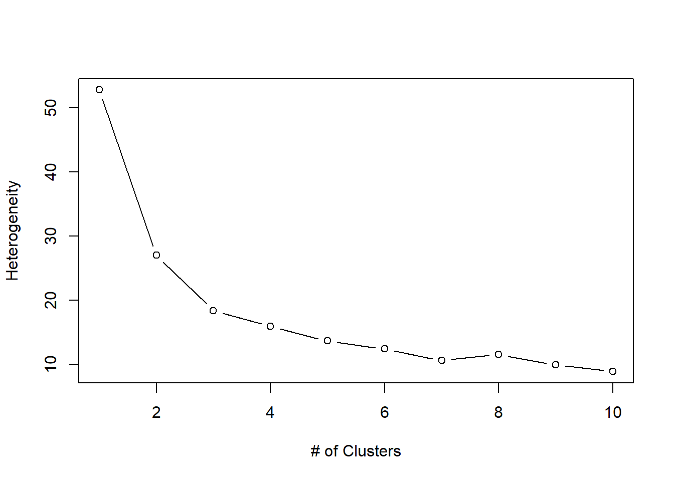
Decide on the best number of clusters:
# optimal number of clusters
c <- 10 # max number for wss-plot
wss <- (nrow(cars2_n)-1)*sum(apply(cars2_n,2,var)); wss[1]
## [1] 52.77075for (i in 2:c) wss[i] <- sum(kmeans(cars2_n, centers=i)$withinss)
plot(1:c, wss, type="b", xlab="# of Clusters", ylab="Heterogeneity")