3 Mapping the Data (by Origin)
3.1 Intro
Let’s display the data on a map.
The leaflet() functions take very long or fail if the number of records is high (on million or so). The data are broken down by six regions.
Below, we take subsets of the data.
We need longitude and latitude, to map the data. But we have longitude and latitude data for both the origin (the sender) and the destination (the receiver). The first subset takes the lat/long of the origin.
The variables are renamed, so that leaflet() will recognize them automatically.
fl_from <- fashlogNum[,c("latfrom","lonfrom","region")]
names(fl_from)[1] <- "lat"
names(fl_from)[2] <- "lon"
head(fl_from)
## lat lon region
## 1 52.35767 6.639536 5
## 2 52.31264 5.034798 1
## 3 52.29684 5.160120 1
## 4 52.29814 6.922199 6
## 5 52.29814 6.922199 2
## 6 52.29814 6.922199 23.2 Region 1
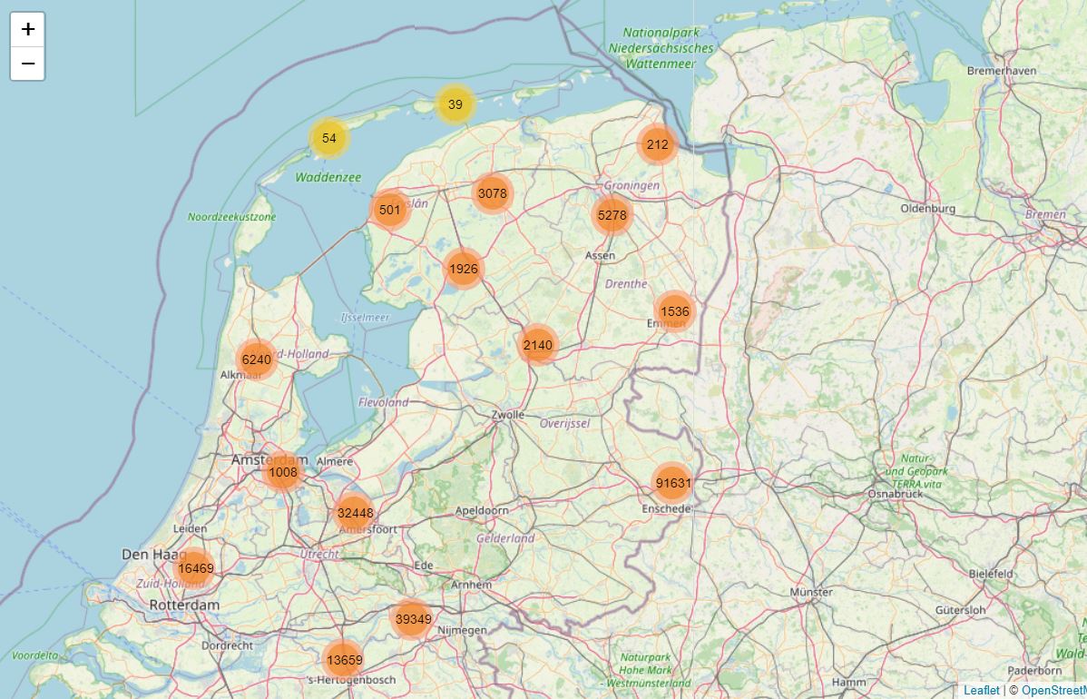
We will now map the number of transactions, in region 1.
library(leaflet)
# Region 1: "From"
# fl_from_r1 <- fl_from[fl_from$region==1,]
# leaflet(fl_from_r1) %>% addTiles() %>% addMarkers(clusterOptions = markerClusterOptions())
If you run the script, you will get a map. Click on the map, and see what happens if you zoom in and out. In your script, of course you have to leave out the #’s that precede the commands!
In order not to slow down this reader, we just show you a screen shot of the map. The numbers in the circles represent the number of shipments.
3.3 Region 2-6
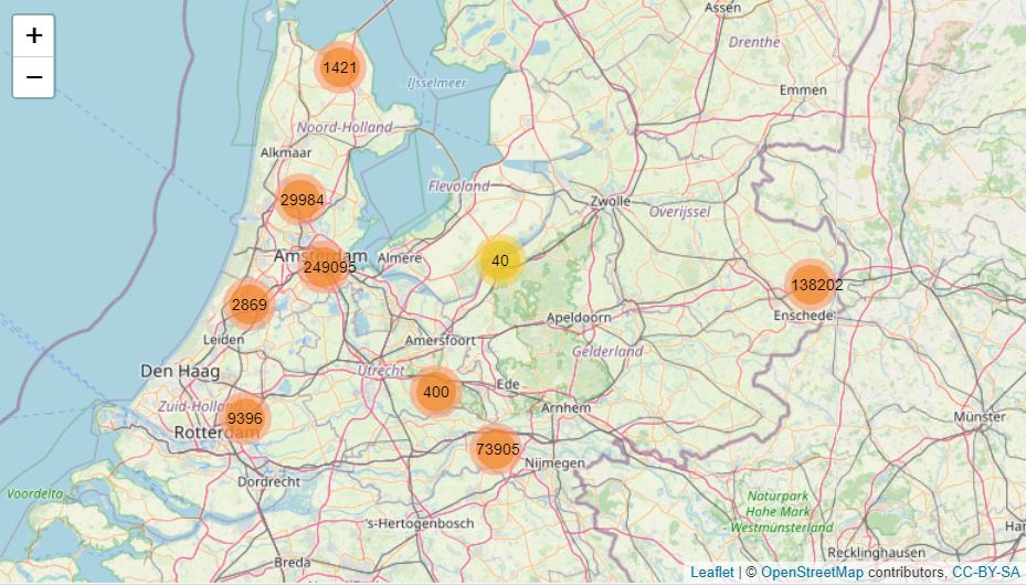
And likewise for region 2, and the other regions.
# Region 2: "From"
# fl_from_r2 <- fl_from[fl_from$region==2,]
# leaflet(fl_from_r2) %>% addTiles() %>% addMarkers(clusterOptions = markerClusterOptions())
Write the script for region 3-5 yourself!
# ... and so on
# Region 6: "From"
# fl_from_r6 <- fl_from[fl_from$region==6,]
# leaflet(fl_from_r6) %>% addTiles() %>% addMarkers(clusterOptions = markerClusterOptions())