5 Describing Distances

Since we are thinking of bundling the goods, in new hubs anywhere in the country or region, it pays off to exclude all transactions over short distances of, say, 20km or 50km.

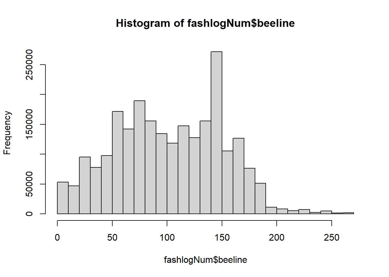
Let’s make an histogram of the “beeline distances,” the straight-line distances between two postal codes.

hist(fashlogNum$beeline)

Simple, but effective.

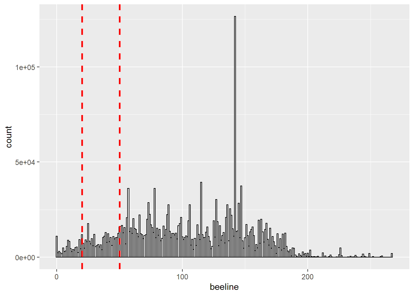
Use ggplot, for fancier graphs.

library(ggplot2)
ggplot(fashlogNum, aes(x=beeline)) + 
  geom_histogram(binwidth=1, colour="black", fill="white") + 
  geom_vline(data=fashlogNum, aes(xintercept=20),
             linetype="dashed", size=1, colour="red") +
  geom_vline(data=fashlogNum, aes(xintercept=50),
             linetype="dashed", size=1, colour="red") 

Rather than graphs, we can do it in numbers. It makes it easier to see how many rides are below 20km, below 50km, and so on.

One option is to create a new variable. We use the dplyr package. We make a new variable with three categories (<20km; 20-<50km; 50+km).

# install.packages("dplyr")
library(dplyr)

## 
## Attaching package: 'dplyr'

## The following objects are masked from 'package:stats':
## 
##     filter, lag

## The following objects are masked from 'package:base':
## 
##     intersect, setdiff, setequal, union

fashlogNum$beelineCat <- case_when((fashlogNum$beeline <= 20) ~ 1,
                  (fashlogNum$beeline >  20) & (fashlogNum$beeline <= 50) ~ 2,
                  (fashlogNum$beeline >  50) ~ 3)
table(fashlogNum$beelineCat)

## 
##       1       2       3 
##  100217  271116 2016108

The table produces numbers. And percentages would be easier.

Below we show (absolute, relative, and cumulative) frequency tables.

The relative and cumulative frequencies are percentages.

distance = fashlogNum$beeline
breaks   = c(0,20,50,100,150,200,250);breaks  

## [1]   0  20  50 100 150 200 250

distance.cut = cut(distance, breaks, right=FALSE)
distance.freq = table(distance.cut)
distance.relfreq = 100*round(distance.freq / nrow(fashlogNum),4)
distance.cumfreq = cumsum(distance.relfreq)
cbind(distance.freq,distance.relfreq,distance.cumfreq)

##           distance.freq distance.relfreq distance.cumfreq
## [0,20)           100217             4.20             4.20
## [20,50)          271116            11.36            15.56
## [50,100)         793051            33.22            48.78
## [100,150)        820510            34.37            83.15
## [150,200)        370765            15.53            98.68
## [200,250)         28280             1.18            99.86