10 OLS Assumptions and Simple Regression Diagnostics
Now that you know how to run and interpret simple regression results, we return to the matter of the underlying assumptions of OLS models, and the steps we can take to determine whether those assumptions have been violated. We begin with a quick review of the conceptual use of residuals, then turn to a set of “visual diagnostics” that can help you identify possible problems in your model. We conclude with a set of steps you can take to address model problems, should they be encountered. As with the previous chapter, we will use examples drawn from the tbur data. As always, we recommend that you try the analyses in the chapter as you read.
10.1 A Recap of Modeling Assumptions
Recall from Chapter 4 that we identified three key assumptions about the error term that are necessary for OLS to provide unbiased, efficient linear estimators; a) errors have identical distributions, b) errors are independent, c) errors are normally distributed.17
Error Assumptions
Errors have identical distributions
\(E(\epsilon^{2}_{i}) = \sigma^2_{\epsilon}\)
Errors are independent of \(X\) and other \(\epsilon_{i}\)
\(E(\epsilon_{i}) \equiv E(\epsilon|x_{i}) = 0\)
and
\(E(\epsilon_{i}) \neq E(\epsilon_{j})\) for \(i \neq j\)
Errors are normally distributed
\(\epsilon_{i} \sim N(0,\sigma^2_{\epsilon})\)
Taken together these assumption mean that the error term has a normal, independent, and identical distribution (normal i.i.d.). Figure 10.1 shows what these assumptions would imply for the distribution of residuals around the predicted values of \(Y\) given \(X\).
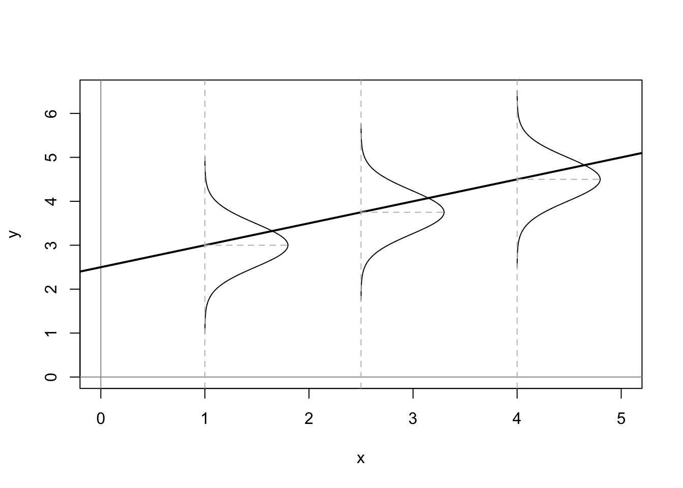
Figure 10.1: Assumed Distributions of OLS Residuals
How can we determine whether our residuals approximate the expected pattern? The most straight-forward approach is to visually examine the distribution of the residuals over the range of the predicted values for \(Y\). If all is well, there should be no obvious pattern to the residuals – they should appear as a “sneeze plot” (i.e., it looks like you sneezed on the plot. How gross!) as shown in Figure 10.2.
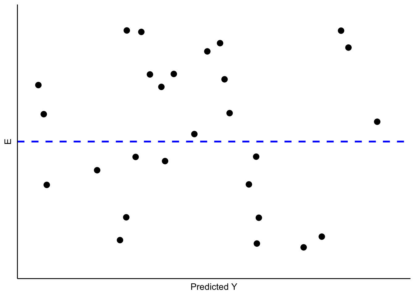
Figure 10.2: Ideal Pattern of Residuals from a Simple OLS Model
Generally, there is no pattern in such a sneeze plot of residuals. One of the difficulties we have, as human beings, is that we tend to look at randomness and perceive patterns. Our brains are wired to see patterns, even where their are none. Moreover, with random distributions there will in some samples be clumps and gaps that do appear to depict some kind of order when in fact there is none. There is the danger, then, of over-interpreting the pattern of residuals to see problems that aren’t there. The key is to know what kinds of patterns to look for, so when you do observe one you will know it.
10.2 When Things Go Bad with Residuals
Residual analysis is the process of looking for signature patterns in the residuals that are indicative of failure in the underlying assumptions of OLS regression. Different kinds of problems lead to different patterns in the residuals.
10.2.1 “Outlier” Data
Sometimes our data include unusual cases that behave differently from most of our observations. This may happen for a number of reasons. The most typical is that the data have been mis-coded, with some subgroup of the data having numerical values that lead to large residuals. Cases like this can also arise when a subgroup of the cases differ from the others in how \(X\) influences \(Y\), and that difference has not been captured in the model. This is a problem referred to as the omission of important independent variables.18 Figure 10.3 shows a stylized example, with a cluster of residuals falling at considerable distance from the rest.
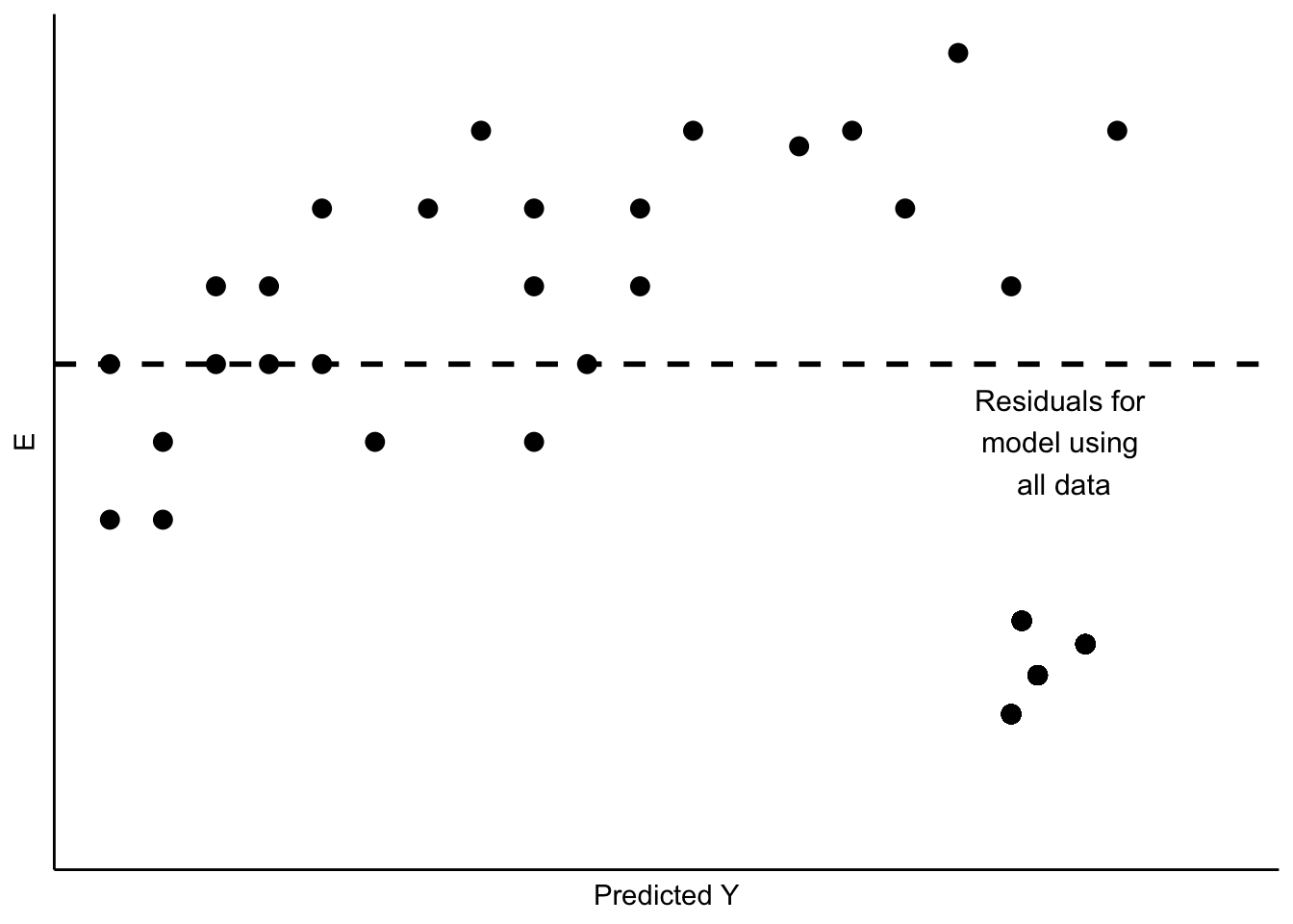
Figure 10.3: Unusual Data Patterns in Residuals
This is a case of influential outliers. The effect of such outliers can be significant, as the OLS estimates of \(A\) and \(B\) seek to minimize overall squared error. In the case of Figure 10.3, the effect would be to shift the estimate of \(B\) to accommodate the unusual observations, as illustrated in Figure 10.4. One possible response would be to omit the unusual observations, as shown in Figure 10.4. Another would be to consider, theoretically and empirically, why these observations are unusual. Are they, perhaps, miscoded? Or are they codes representing missing values (e.g., “-99”)?
If they are not mis-codes, perhaps these outlier observations manifest a different kind of relationship between \(X\) and \(Y\), which might in turn require a revised theory and model. We will address some modeling options to address this possibility when we explore multiple regression, in Part III of this book.
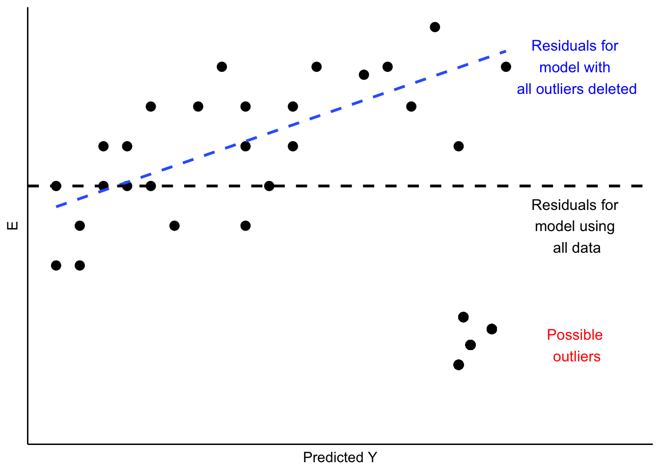
Figure 10.4: Implications of Unusual Data Patterns in Residuals
In sum, outlier analysis looks at residuals for patterns in which some observations deviate widely from others. If that deviation is influential, changing estimates of \(A\) and \(B\) as shown in Figure 10.4, then you must examine the observations to determine whether they are mis-coded. If not, you can evaluate whether the cases are theoretically distinct, such that the influence of \(X\) on \(Y\) is likely to be different than for other cases. If you conclude that this is so, you will need to respecify your model to account for these differences. We will discuss some options for doing that later in this chapter, and again in our discussion of multiple regression.
10.2.2 Non-Constant Variance
A second thing to look for in visual diagnostics of residuals is non-constant variance, or heteroscedasticity. In this case, the variation in the residuals over the range of predicted values for \(Y\) should be roughly even. A problem occurs when that variation changes substantially as the predicted value of \(Y\) changes, as is illustrated in Figure 10.5.
##    x5           y5    z5
## 1   1  0.116268529 first
## 2   2 -0.058592447 first
## 3   3  0.178546500 first
## 4   4 -0.133259371 first
## 5   5 -0.044656677 first
## 6   6  0.056960612 first
## 7   7 -0.288971761 first
## 8   8 -0.086901834 first
## 9   9 -0.046170268 first
## 10 10 -0.055554091 first
## 11 11 -0.002013537 first
## 12 12 -0.015038222 first
## 13 13 -0.062812676 first
## 14 14  0.132322085 first
## 15 15 -0.152135057 first
## 16 16 -0.043742787 first
## 17 17  0.097057758 first
## 18 18  0.002822264 first
## 19 19 -0.008578219 first
## 20 20  0.038921440 first
## 21 21  0.023668737 first
## x5 y5 z5
## 1 21 -0.7944212 second
## 2 22 3.9722634 second
## 3 23 2.0344877 second
## 4 24 -1.3313647 second
## 5 25 -8.0963483 second
## 6 26 -3.2788775 second
## 7 27 -6.3068507 second
## 8 28 -13.6105004 second
## 9 29 -3.3742972 second
## 10 30 -1.1897133 second
## 11 31 8.7458017 second
## 12 32 8.5587880 second
## 13 33 6.0964799 second
## 14 34 -6.0353801 second
## 15 35 -10.2333314 second
## 16 36 -5.0246837 second
## 17 37 6.8506290 second
## 18 38 0.4832010 second
## 19 39 2.3291504 second
## 20 40 -4.5016566 second
## 21 41 -8.4841231 second## x5 y5 z5
## 1 1 0.116268529 first
## 2 2 -0.058592447 first
## 3 3 0.178546500 first
## 4 4 -0.133259371 first
## 5 5 -0.044656677 first
## 6 6 0.056960612 first
## 7 7 -0.288971761 first
## 8 8 -0.086901834 first
## 9 9 -0.046170268 first
## 10 10 -0.055554091 first
## 11 11 -0.002013537 first
## 12 12 -0.015038222 first
## 13 13 -0.062812676 first
## 14 14 0.132322085 first
## 15 15 -0.152135057 first
## 16 16 -0.043742787 first
## 17 17 0.097057758 first
## 18 18 0.002822264 first
## 19 19 -0.008578219 first
## 20 20 0.038921440 first
## 21 21 0.023668737 first
## 22 21 -0.794421247 second
## 23 22 3.972263354 second
## 24 23 2.034487716 second
## 25 24 -1.331364730 second
## 26 25 -8.096348251 second
## 27 26 -3.278877502 second
## 28 27 -6.306850722 second
## 29 28 -13.610500382 second
## 30 29 -3.374297181 second
## 31 30 -1.189713327 second
## 32 31 8.745801727 second
## 33 32 8.558788016 second
## 34 33 6.096479914 second
## 35 34 -6.035380147 second
## 36 35 -10.233331440 second
## 37 36 -5.024683664 second
## 38 37 6.850629016 second
## 39 38 0.483200951 second
## 40 39 2.329150423 second
## 41 40 -4.501656591 second
## 42 41 -8.484123104 second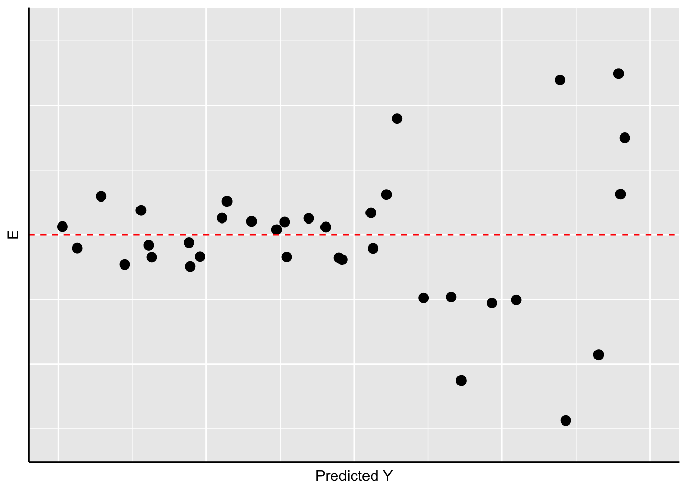
Figure 10.5: Non-Constant Variance in the Residuals
As Figure 10.5 shows, the width of the spread of the residuals grows as the predicted value of \(Y\) increases, making a fan-shaped pattern. Equally concerning would be a case of a “reverse fan”, or a pattern with a bulge in the middle and very “tight” distributions of residuals at either extreme. These would all be cases in which the assumption of constant-variance in the residuals (or “homoscedasticity”) fails, and are referred to as instances of heteroscedasticity.
What are the implications of heteroscedasticity? Our hypothesis tests for the estimated coefficients (\(A\) and \(B\)) are based on the assumption that the standard errors of the estimates (see the prior chapter) are normally distributed. If inspection of your residuals provides evidence to question that assumption, then the interpretation of the t-values and p-values may be problematic. Intuitively, in such a case the precision of our estimates of \(A\) and \(B\) are not constant – but rather will depend on the predicted value of \(Y\). So you might be estimating \(B\) relatively precisely in some ranges of \(Y\), and less precisely in others. That means you cannot depend on the estimated t and p-values to test your hypotheses.
10.2.3 Non-Linearity in the Parameters
One of the primary assumptions of simple OLS regression is that the estimated slope parameter (the \(B\)) will be constant, and therefore the model will be linear. Put differently, the effect of any change in \(X\) on \(Y\) should be constant over the range of \(Y\). Thus, if our assumption is correct, the pattern of the residuals should be roughly symmetric, above and below zero, over the range of predicted values.
If the real relationship between \(X\) and \(Y\) is not linear, however, the predicted (linear) values for \(Y\) will systematically depart from the (curved) relationship that is represented in the data. Figure 10.6 shows the kind of pattern we would expect in our residuals if the observed relationship between \(X\) and \(Y\) is a strong curve, when we attempt to model it as if it were linear.
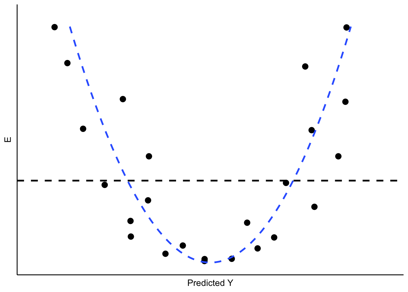
Figure 10.6: Non-Linearity in the Residuals
What are the implications of non-linearity? First, because the slope is non-constant, the estimate of \(B\) will be biased. In the illustration shown in Figure 10.6, \(B\) would underestimate the value of \(Y\) in both the low and high ranges of the predicted value of \(Y\), and overestimate it in the mid-range. In addition, the standard errors of the residuals will be large, due to systematic over- and under-estimation of \(Y\), making the model very inefficient (or imprecise).
10.3 Application of Residual Diagnostics
This far we have used rather simple illustrations of residual diagnostics and the kinds of patterns to look for. But you should be warned that, in real applications, the patterns are rarely so clear. So we will walk through an example diagnostic session, using the the tbur data set.
Our in-class lab example focuses on the relationship between political ideology (“ideology” in our dataset) as a predictor of the perceived risks posed by climate change (“gccrsk”). The model is specified in R as follows:
Using the summary command in R, we can review the results.
##
## Call:
## lm(formula = ds$glbcc_risk ~ ds$ideol)
##
## Residuals:
##    Min     1Q Median     3Q    Max
## -8.726 -1.633  0.274  1.459  6.506
##
## Coefficients:
##             Estimate Std. Error t value Pr(>|t|)
## (Intercept) 10.81866    0.14189   76.25   <2e-16 ***
## ds$ideol    -1.04635    0.02856  -36.63   <2e-16 ***
## ---
## Signif. codes:  0 '***' 0.001 '**' 0.01 '*' 0.05 '.' 0.1 ' ' 1
##
## Residual standard error: 2.479 on 2511 degrees of freedom
##   (34 observations deleted due to missingness)
## Multiple R-squared:  0.3483, Adjusted R-squared:  0.348
## F-statistic:  1342 on 1 and 2511 DF,  p-value: < 2.2e-16
Note that, as was discussed in the prior chapter, the estimated value for \(B\) is negative and highly statistically significant. This indicates that the more conservative the survey respondent, the lower the perceived risks attributed to climate change. Now we will use these model results and the associated residuals to evaluate the key assumptions of OLS, beginning with linearity.
10.3.1 Testing for Non-Linearity
One way to test for non-linearity is to fit the model to a polynomial functional form. This sounds impressive, but is quite easy to do and understand (really!). All you need to do is include the square of the independent variable as a second predictor in the model. A significant regression coefficient on the squared variable indicates problems with linearity. To do this, we first produce the squared variable.
#first we square the ideology variable and create a new variable to use in our model.
ds$ideology2 <- ds$ideol^2
summary(ds$ideology2)
## Min. 1st Qu. Median Mean 3rd Qu. Max. NA's
## 1.00 16.00 25.00 24.65 36.00 49.00 23Next, we run the regression with the original independent variable and our new squared variable. Finally, we check the regression output.
OLS_env2 <- lm(glbcc_risk ~ ideol + ideology2, data = ds)
summary(OLS_env2)
A significant coefficient on the squared ideology variable informs us that we probably have a non-linearity problem. The significant and negative coefficient for the square of ideology means that the curve steepens (perceived risks fall faster) as the scale shifts further up on the conservative side of the scale. We can supplement the polynomial regression test by producing a residual plot with a formal Tukey test. The residual plot (car package residualPlots function) displays the Pearson fitted values against the model’s observed values. Ideally, the plots will produce flat red lines; curved lines represent non-linearity. The output for the Tukey test is visible in the \(R\) workspace. The null hypothesis for the Tukey test is a linear relationship, so a significant p-value is indicative of non-linearity. The tukey test is reported as part of the residualPlots function in the car package.
#A significant p-value indicates non-linearity using the Tukey test
library(car)
residualPlots(OLS_env)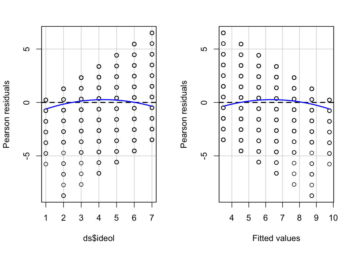
Figure 10.7: Residual Plots Examining Model Linearity
##            Test stat Pr(>|Test stat|)
## ds$ideol     -5.0181        5.584e-07 ***
## Tukey test   -5.0181        5.219e-07 ***
## ---
## Signif. codes:  0 '***' 0.001 '**' 0.01 '*' 0.05 '.' 0.1 ' ' 1
The curved red lines in Figure 10.7 in the residual plots and significant Tukey test indicate a non-linear relationship in the model. This is a serious violation of a core assumption of OLS regression, which means that the estimate of \(B\) is likely to be biased. Our findings suggest that the relationship between ideology and perceived risks of climate change is approximately linear from “strong liberals” to those who are “leaning Republican”. But perceived risks seem to drop off more rapidly as the scale rises toward “strong Republican.”
10.3.2 Testing for Normality in Model Residuals
Testing for normality in the model residuals will involve using many of the techniques demonstrated in previous chapters. The first step is to graphically display the residuals in order to see how closely the model residuals resemble a normal distribution. A formal test for normality is also included in the demonstration.
Start by creating a histogram of the model residuals.
OLS_env$residuals %>% # Pipe the residuals to a data frame
  data.frame() %>% # Pipe the data frame to ggplot
  ggplot(aes(OLS_env$residuals)) +
  geom_histogram(bins = 16)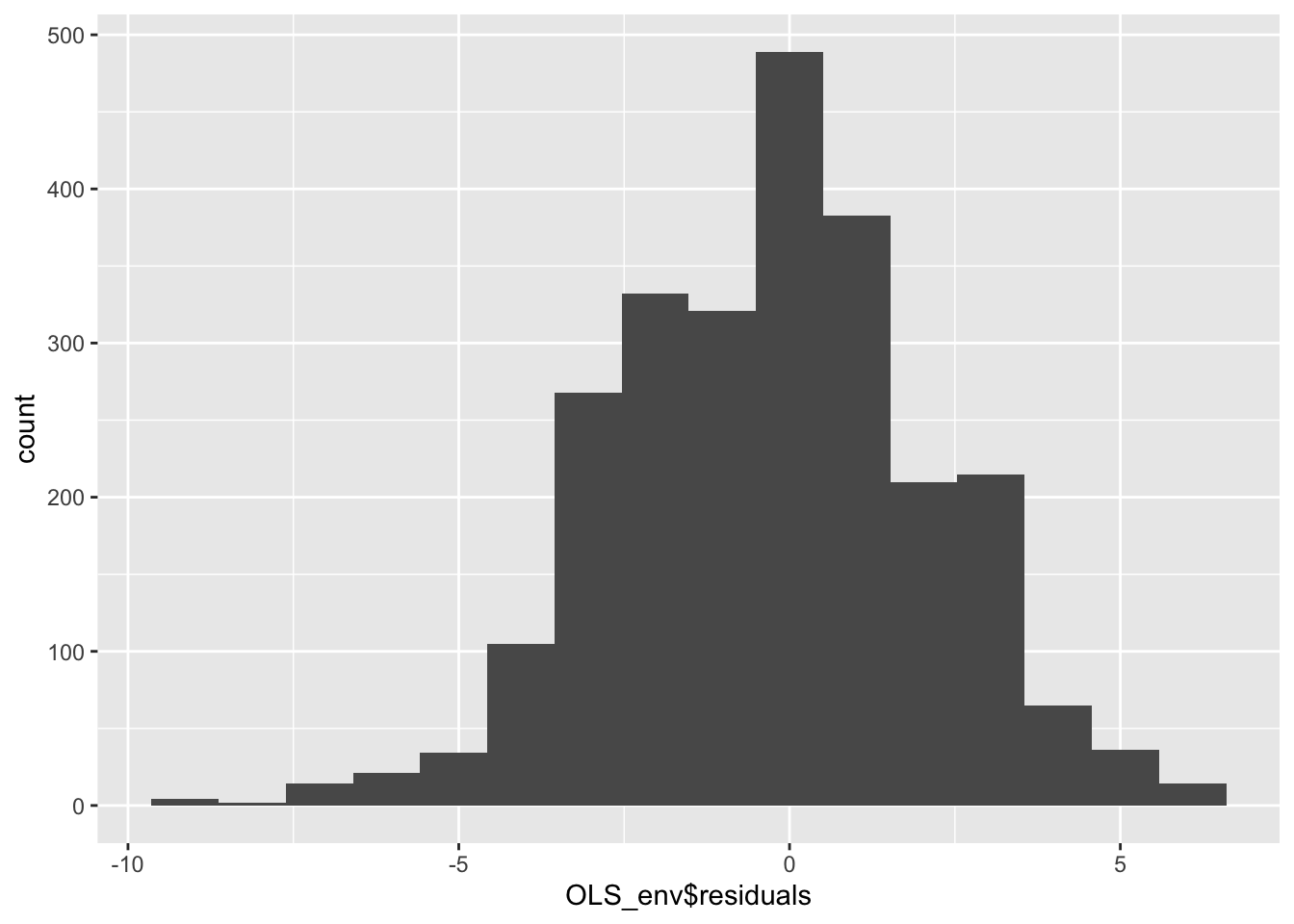
Figure 10.8: Histogram of Model Residuals
The histogram in figure 10.8 indicates that the residuals are approximately normally distributed, but there appears to be a negative skew. Next, we can create a smoothed density of the model residuals compared to a theoretical normal distribution.
OLS_env$residuals %>% # Pipe the residuals to a data frame
  data.frame() %>% # Pipe the data frame to ggplot
  ggplot(aes(OLS_env$residuals)) +
  geom_density(adjust = 2) +
  stat_function(fun = dnorm, args = list(mean = mean(OLS_env$residuals),
                                         sd = sd(OLS_env$residuals)),
                color = "red")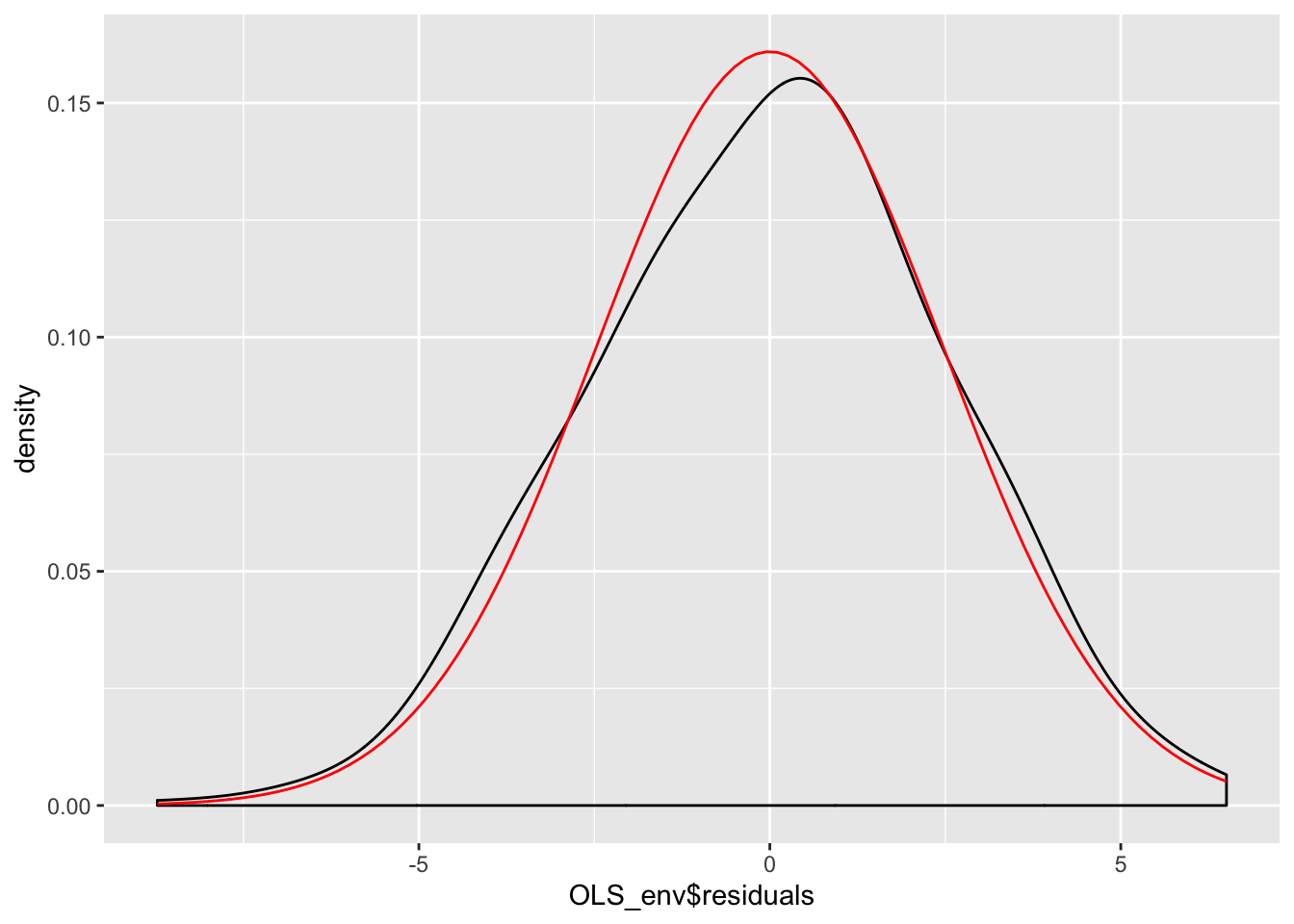
Figure 10.9: Smoothed Density Plot of Model Residuals
Figure 10.9 indicates the model residuals deviate slightly from a normal distributed because of a slightly negative skew and a mean higher than we would expect in a normal distribution. Our final ocular examination of the residuals will be a quartile plot %(using the stat_qq function from the ggplot2 package).
OLS_env$residuals %>% # Pipe the residuals to a data frame
  data.frame() %>% # Pipe the data frame to ggplot
  ggplot(aes(sample = OLS_env$residuals)) +
  stat_qq() +
  stat_qq_line()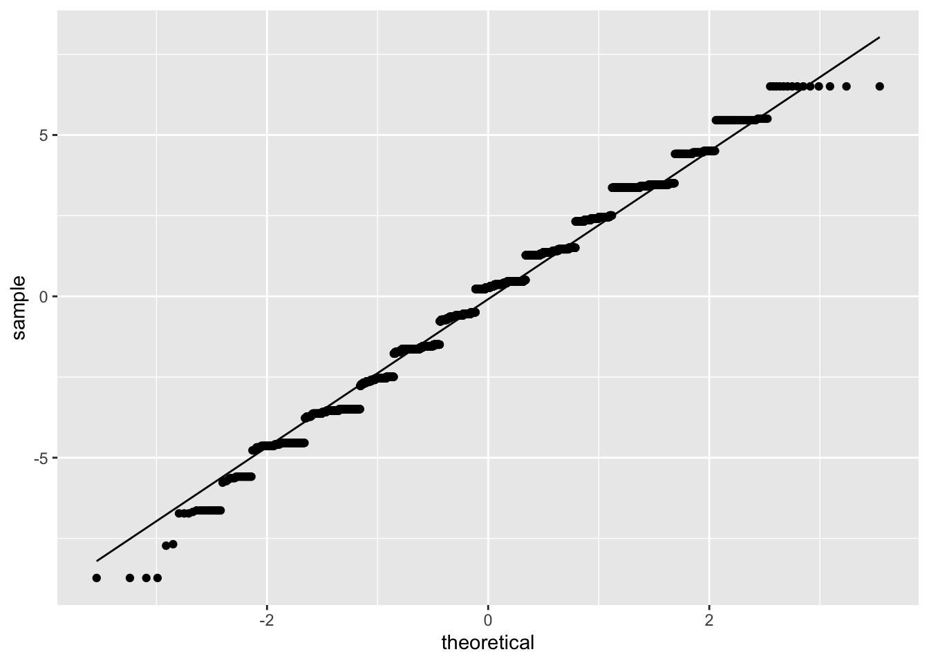
Figure 10.10: Quartile Plot of Model Residuals
According to Figure 10.10, it appears as if the residuals are normally distributed except for the tails of the distribution. Taken together the graphical representations of the residuals suggest modest non-normality. As a final step, we can conduct a formal Shapiro-Wilk test for normality. The null hypothesis for a Shapiro-Wilk test is a normal distribution, so we do not want to see a significant p-value.
#a significant value p-value potentially indicates the data is not normally distributed.
shapiro.test(OLS_env$residuals)
##
## Shapiro-Wilk normality test
##
## data: OLS_env$residuals
## W = 0.98901, p-value = 5.51e-13The Shapiro-Wilk test confirms what we observed in the graphical displays of the model residuals – the residuals are not normally distributed. Recall that our dependent variable (gccrsk) appears to have a non-normal distribution. This could be the root of the non-normality found in the model residuals. Given this information, steps must be taken to assure that the model residuals meet the required OLS assumptions. One possibility would be to transform the dependent variable (glbccrisk) in order to induce a normal distribution. Another might be to add a polynomial term to the independent variable (ideology) as was done above. In either case, you would need to recheck the residuals in order to see if the model revisions adequately dealt with the problem. We suggest that you do just that!
10.3.3 Testing for Non-Constant Variance in the Residuals
Testing for non-constant variance (heteroscedasticity) in a model is fairly straightforward. We can start by creating a spread-level plot that fits the studentized residuals against the model’s fitted values. A line with a non-zero slope is indicative of heteroscedasticity. Figure 10.11 displays the spread-level plot from the car package.
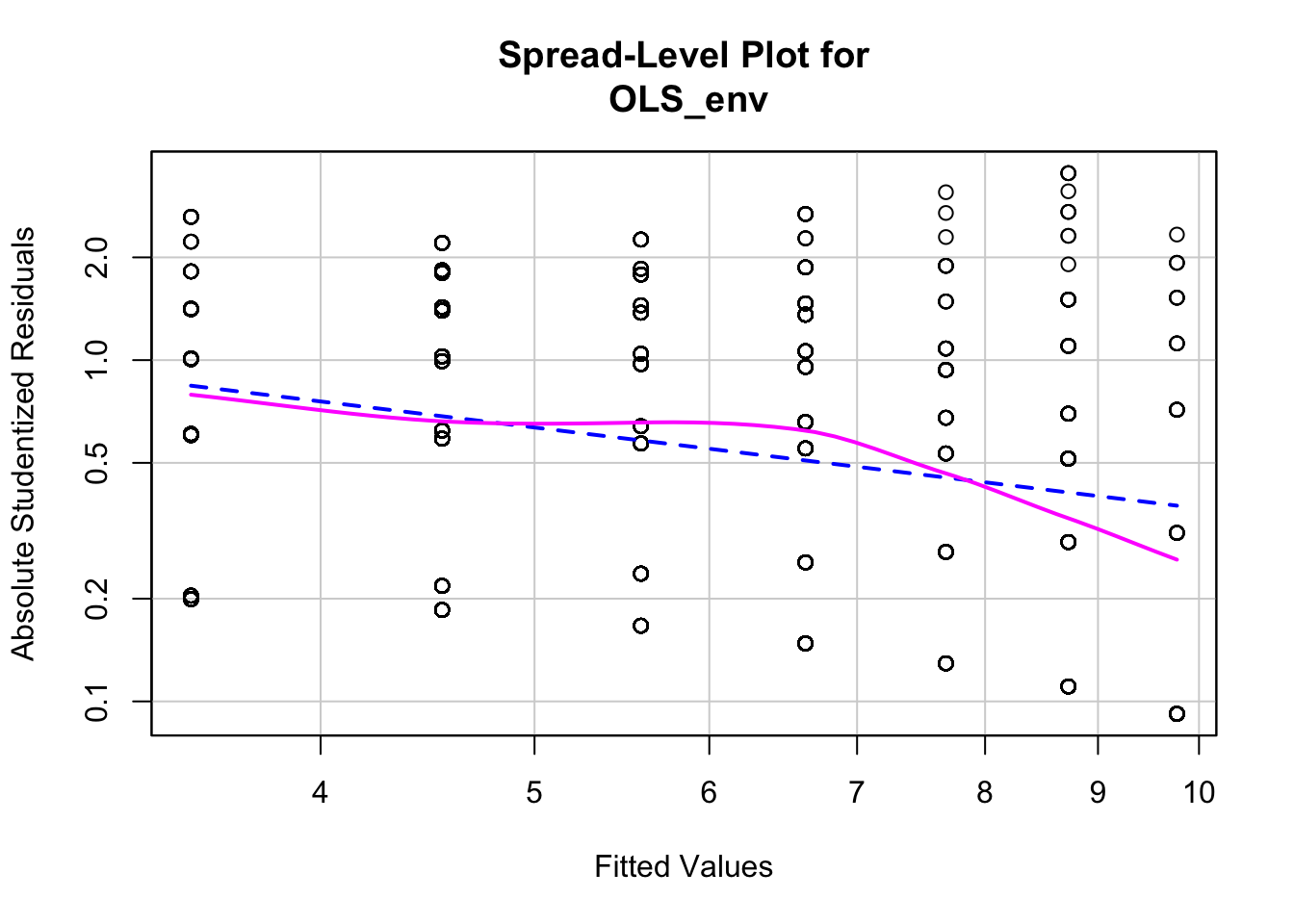
Figure 10.11: Spread-Level Plot of Model Residuals
##
## Suggested power transformation: 1.787088## null device
## 1The negative slope on the red line in Figure 10.11 indicates the model may contain heteroscedasticity. We can also perform a formal test for non constant variance. The null hypothesis is constant variance, so we do not want to see a significant p-value.
## Non-constant Variance Score Test
## Variance formula: ~ fitted.values
## Chisquare = 68.107, Df = 1, p = < 2.22e-16
The significant p-value on the non-constant variance test informs us that there is a problem with heteroscedasticity in the model. This is yet another violation of the core assumptions of OLS regression, and it brings into doubt our hypothesis tests.
10.3.4 Examining Outlier Data
There are a number of ways to examine outlying observations in an OLS regression. This section briefly illustrates a a subset of analytical tests that will provide a useful assessment of potentially important outliers. The purpose of examining outlier data is twofold. First, we want to make sure there are not any mis-coded or invalid data influencing our regression. For example, an outlying observation with a value of “-99” would very likely bias our results, and obviously needs to be corrected. Second, outlier data may indicate the need to theoretically reconceptualize our model. Perhaps the relationship in the model is mis-specified, with outliers at the extremes of a variable suggesting a non-linear relationship. Or it may be that a subset of cases respond differently to the independent variable, and therefore must be treated as “special cases” in the model. Examining outliers allows us to identify and address these potential problems.
One of the first things we can do is perform a Bonferroni Outlier Test. The Bonferroni Outlier Tests uses a \(t\) distribution to test whether the model’s largest studentized residual value’s outlier status is statistically different from the other observations in the model. A significant p-value indicates an extreme outlier that warrants further examination. We use the outlierTest function in the car package to perform a Bonferroni Outlier Test.
## No Studentized residuals with Bonferroni p < 0.05
## Largest |rstudent|:
##      rstudent unadjusted p-value Bonferroni p
## 589 -3.530306         0.00042255           NA
According to the R output, the Bonferroni p-value for the largest (absolute) residual is not statistically significant. While this test is important for identifying a potentially significant outlying observation, it is not a panacea for checking for patterns in outlying data. Next we will examine the model’s df.betas in order to see which observations exert the most influence on the model’s regression coefficients. \(Dfbetas\) are measures of how much the regression coefficient changes when observation \(i\) is omitted. Larger values indicate an observation that has considerable influence on the model.
A useful method for finding dfbeta obervations is to use the dfbetaPlots function in the car package. We specify the option id.n=2 to show the two largest df.betas. See figure 10.12.
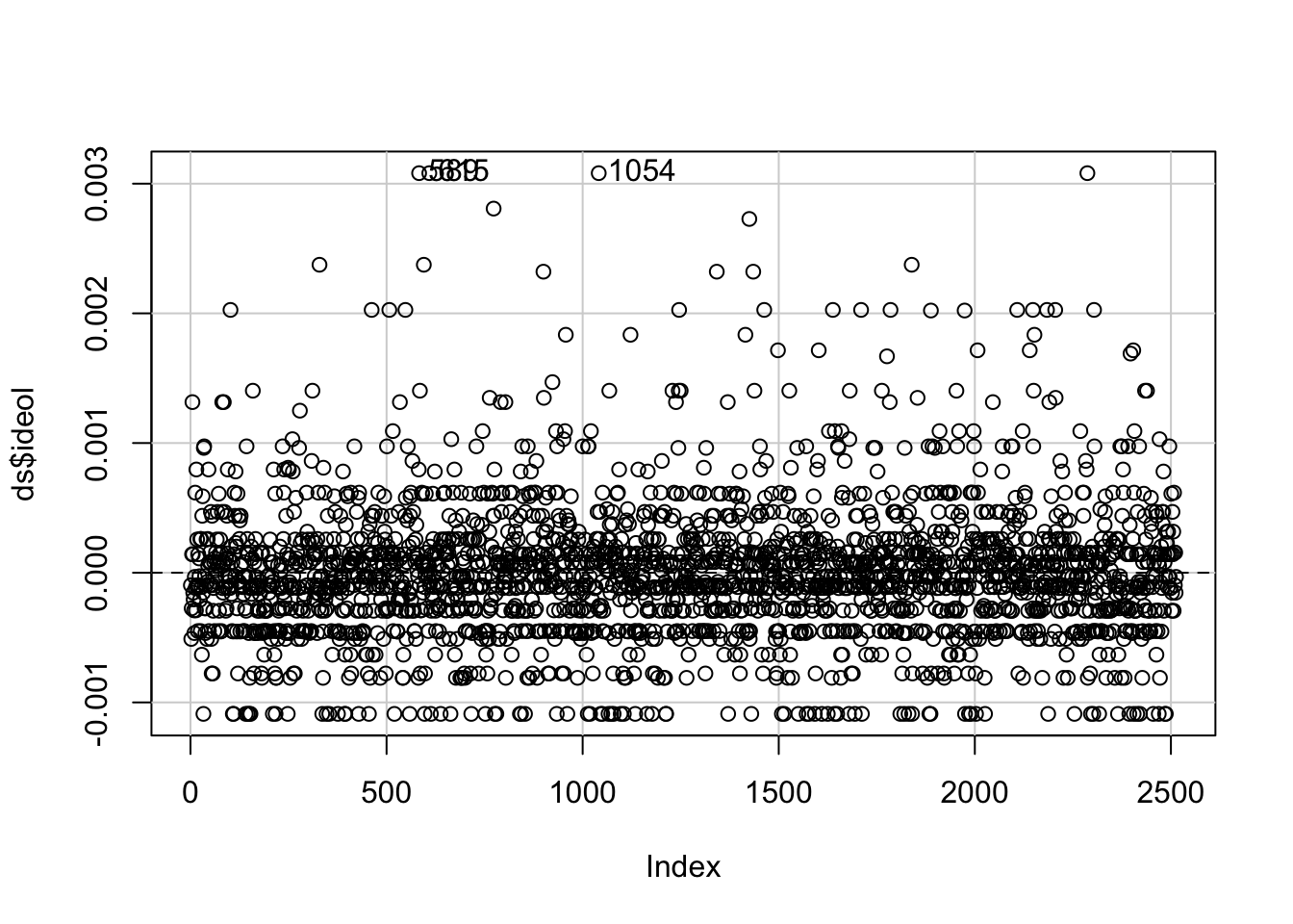
Figure 10.12: Plot of Model dfbetas Values using ‘dfbetaPlots’ function
#  Check the observations with high dfbetas.
#  We see the values 589 and 615 returned.
#  We only want to see results from columns gccrsk and ideology in tbur.data.
ds[c(589,615),c("glbcc_risk", "ideol")]
## glbcc_risk ideol
## 589 0 2
## 615 0 2These observations are interesting because they identify a potential problem in our model specification. Both observations are considered outliers because the respondents self-identified as “liberal” (ideology = 1) and rated their perceived risk of global climate change as 0. These values deviate substantially from the norm for other strong liberals in the dataset. Remember, as we saw earlier, our model has a problem with non-linearity – these outlying observations seem to corroborate this finding. Examination of outliers sheds some light on the issue.
Finally, we can produce a plot that combines studentized residuals, “hat values”, and Cook’s D distances (these are measures of the amount of influence observations have on the model) using circles as an indicator of influence – the larger the circle, the greater the influence. Figure 10.13 displays the combined influence plot. In addition, the influencePlot function returns the values of greatest influence.
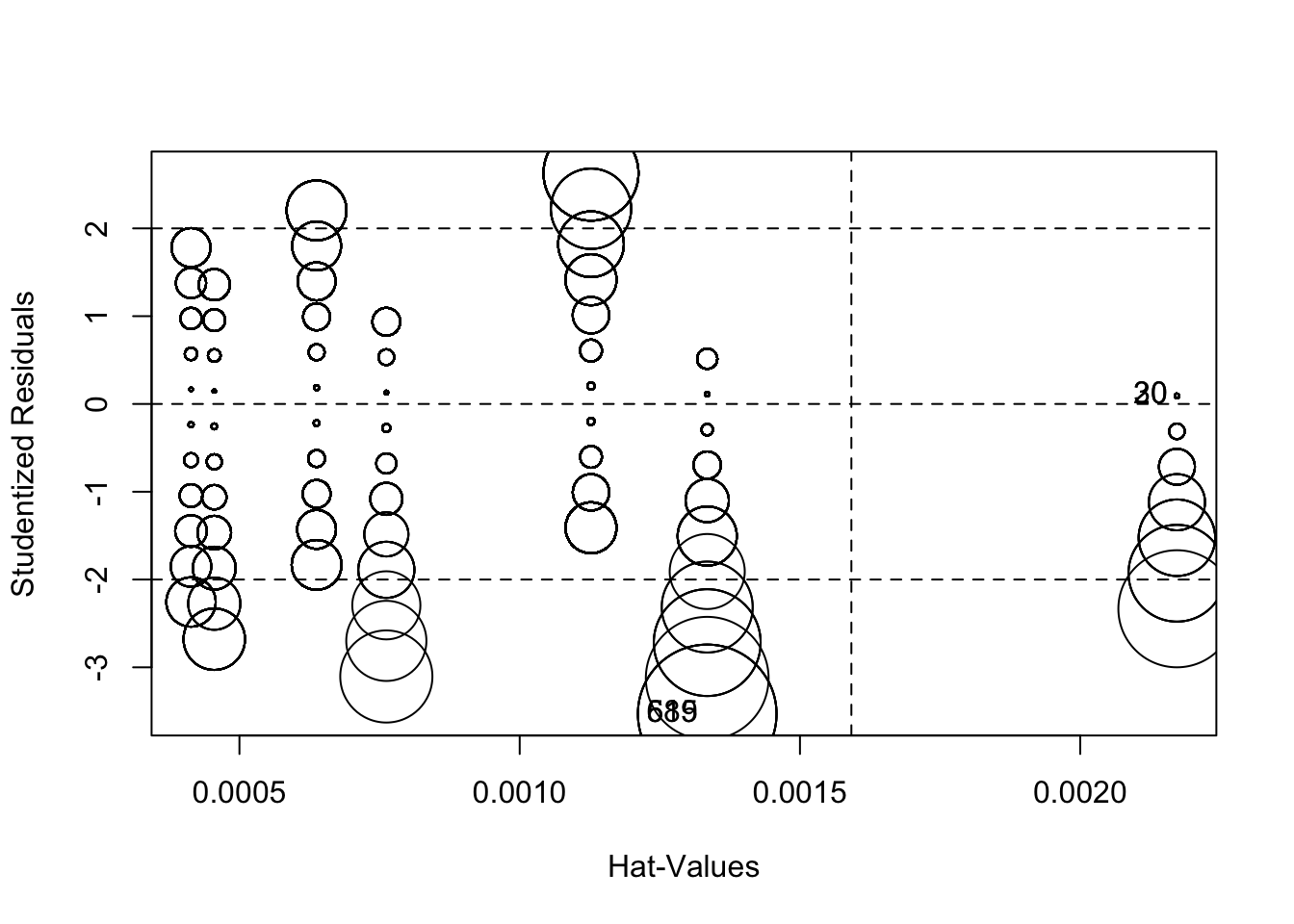
Figure 10.13: Influence Bubble Plot
## StudRes Hat CookD
## 20 0.09192603 0.002172497 9.202846e-06
## 30 0.09192603 0.002172497 9.202846e-06
## 589 -3.53030574 0.001334528 8.289419e-03
## 615 -3.53030574 0.001334528 8.289419e-03Figure 10.13 indicates that there are a number of cases that warrant further examination. We are already familiar with 589 and 615 Let’s add 20, 30, 90 and 1052.
##     glbcc_risk ideol
## 589          0     2
## 615          0     2
## 20 10 1
## 30 10 1
## 90 10 1
## 1052 3 6One important take-away from a visual examination of these observations is that there do not appear to be any completely mis-coded or invalid data affecting our model. In general, even the most influential observations do not appear to be implausible cases. Observations 589 and 615 19 present an interesting problem regarding theoretical and model specification. These observations represent respondents who self-reported as “liberal” (ideology=2) and also rated the perceived risk of global climate change as 0 out of 10. These observations therefore deviate from the model’s expected values (“strong liberal” respondents, on average, believed global climate change represents a high risk). Earlier in our diagnostic testing we found a problem with non-linearity. Taken together, it looks like the non-linearity in our model is due to observations at the ideological extremes. One way we can deal with this problem is to include a squared ideology variable (a polynomial) in the model, as illustrated earlier in this chapter. However, it is also important to note this non-linear relationship in the theoretical conceptualization of our model. Perhaps there is something special about people with extreme ideologies that needs to be taken into account when attempting to predict perceived risk of global climate change. This finding should also inform our examination of post-estimation predictions – something that will be covered later in this text.
10.4 So Now What? Implications of Residual Analysis
What should you do if you observe patterns in the residuals that seem to violate the assumptions of OLS? If you find deviant cases – outliers that are shown to be highly influential – you need to first evaluate the specific cases (observations). Is it possible that the data were miscoded? We hear of many instances in which missing value codes (often “-99”) were inadvertently left in the dataset. R would treat such values as if they were real data, often generating glaring and influential outliers. Should that be the case, recode the offending variable observation as missing (“NA”) and try again.
But what if there is no obvious coding problem? It may be that the influential outlier is appropriately measured, but that the observation is different in some theoretically important way. Suppose, for example, that your model included some respondents who – rather than diligently answering your questions – just responded at random to your survey questions. They would introduce noise and error. If you could measure these slackers, you could either exclude them or include a control variable in your model to account for their different patterns of responses. We will discuss inclusion of model controls when we turn to multiple regression modeling in later chapters.
What if your residual analysis indicates the presence of heteroscedasticity? Recall that this will undermine your ability to do hypothesis tests in OLS. There are several options. If the variation in fit over the range of the predicted value of \(Y\) could plausibly result from the omission of an important explanatory variable, you should respecify your model accordingly (more on this later in this book). It is often the case that you can improve the distribution of residuals by including important but previously omitted variables. Measures of income, when left out of consumer behavior models, often have this effect.
Another approach is to use a different modeling approach that accounts for the heteroscedasticity in the estimated standard error. Of particular utility are robust estimators, which can be employed using the rlm (robust linear model) function in the MASS package. This approach increases the magnitude of the estimated standard errors, reducing the t-values and resulting p-values. That means that the “cost” of running robust estimators is that the precision of the estimates is reduced.
Evidence of non-linearity in the residuals presents a thorny problem. This is a basic violation of a central assumption of OLS, resulting in biased estimates of \(A\) and \(B\). What can you do? First, you can respecify your model to include a polynomial; you would include both the \(X\) variable and a square of the \(X\) variable. Note that this will require you to recode \(X\). In this approach, the value of \(X\) is constant, while the value of the square of \(X\) increases exponentially. So a relationship in which \(Y\) decreases as the square of \(X\) increases will provide a progressively steeper slope as \(X\) rises. This is the kind of pattern we observed in the example in which political ideology was used to predict the perceived risk posed by climate change.
10.5 Summary
Now you are in a position to employ diagnostics – both visual and statistical – to evaluate the results of your statistical models. Note that, once you have made your model corrections, you will need to regenerate and re-evaluate your model residuals to determine whether the problem has been ameliorated. Think of diagnostics as an iterative process in which you use the model results to evaluate, diagnose, revise re-run, and re-evaluate your model. This is where the real learning happens, as you challenge your theory (as specified in your model) with observed data. So – have at it!
Again, we assume only that the means of the errors drawn from repeated samples of observations will be normally distributed – but we will often find that errors in a particular sample deviate significantly from a normal distribution.↩
Political scientists who study US electoral politics have had to account for unusual observations in the Southern states. Failure in the model to account for these differences would lead to prediction error and ugly patterns in the residuals. Sadly, Professor Gaddie notes that scholars have not been sufficiently careful – or perhaps well-trained? – to do this right. Professor Gaddie notes: “… instead of working to achieve better model specification through the application of theory and careful thought, in the 1960s and 1970s electoral scholars instead just threw out the South and all senate races, creating the perception that the United States had 39 states and a unicameral legislature.”↩
Of note, observations 20, 30, and 90 and 1052 are returned as well. There doesn’t appear to be anything special about these four observations. Part of this may be due to the bivariate relationship and how the
influcencePlotfunction weights the data. The results are included for your review.↩