8 Linear Estimation and Minimizing Error
As noted in the last chapter, the objective when estimating a linear model is to minimize the aggregate of the squared error. Specifically, when estimating a linear model, \(Y=A+BX+E\), we seek to find the values of \(\hat{\alpha}\) and \(\hat{\beta}\) that minimize the \(\sum \epsilon^{2}\). To accomplish this, we use calculus.
8.1 Minimizing Error using Derivatives
In calculus, the derivative is a measure the slope of any function of x, or \(f(x)\), at each given value of \(x\). For the function \(f(x)\), the derivative is denoted as \(f'(x)\) or, pronounced as “f prime x”. Because the formula for \(\sum \epsilon^{2}\) is known, and can be treated as a function, the derivative of that function permits the calculation of the change in the sum of the squared error over each possible value of \(\hat{\alpha}\) and \(\hat{\beta}\). For that reason we need to find the derivative for \(\sum \epsilon^{2}\) with respect to changes in \(\hat{\alpha}\) and \(\hat{\beta}\). That, in turn, will permit us to “derive” the values of \(\hat{\alpha}\) and \(\hat{\beta}\) that result in the lowest possible \(\sum \epsilon^{2}\).
Look – we understand that this all sounds complicated. But it’s not all that complicated. In this chapter we will walk through all the steps so you’ll see that its really rather simple and, well, elegant. You will see that differential calculus (the kind of calculus that is concerned with rates of change) is built on a set of clearly defined rules for finding the derivative for any function \(f(x)\). It’s like solving a puzzle. The next section outlines these rules, so we can start solving puzzles.
8.1.1 Rules of Derivation
Derivative Rules
- Power Rule
- Constant Rule
- A Constant Times a Function
- Differentiating a Sum
- Product Rule
- Quotient Rule
- Chain Rule
The following sections provide examples of the application of each rule.
Rule 1: The Power Rule
Example: \[\begin{align*} f(x) &= x^{6} \\ f'(x) &= 6*x^{6-1} \\ &=6x^{5} \end{align*}\]
A second example can be plotted in R. The function is \(f(x)=x^{2}\) and therefore, using the power rule, the derivative is: \(f'(x)=2x\).
## [1] -5 -4 -3 -2 -1 0 1 2 3 4 5## [1] 25 16 9 4 1 0 1 4 9 16 25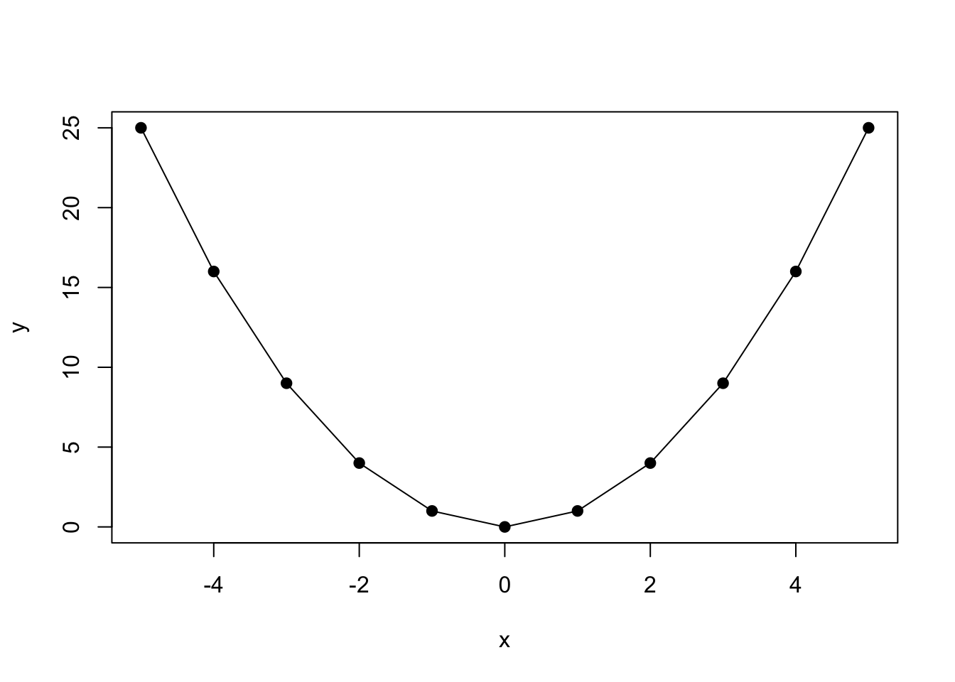
Figure 8.1: Calculating Slopes for \((x,y)\) Pairs
Rule 2: The Constant Rule
Example: \[\begin{align*} f(x) &=346 \\ f'(x)&=0 \\ &=10x \end{align*}\]
Rule 3: A Constant Times a Function
Example: \[\begin{align*} f(x) &= 5x^{2} \\ f'(x)&=5*2x^{2-1} \\ &=10x \end{align*}\]
Rule 4: Differentiating a Sum
Example:
\[\begin{align*}
f(x)&= 4x^{2}+32x \\
f'(x)&=(4x^{2})'+(32x)' \\
&=4*2x^{2-1}+32 \\
&=8x+32
\end{align*}\]
Rule 5: The Product Rule
Example: \[\begin{align*} f(x) &= x^{3}(x-5) \\ f'(x)&=(x^{3})'(x-5)+(x^{3})(x-5)' \\ &=3x^{2}(x-5)+(x^{3})*1 \\ &=3x^{3}-15x^{2}+x^{3}\\ &=4x^{3}-15x^{2} \end{align*}\]
In a second example, the product rule is applied to the function \(y=f(x)=x^{2}-6x+5\). The derivative of this function is \(f'(x)=2x-6\). This function can be plotted in R.
## [1] -1 0 1 2 3 4 5 6 7## [1] 12 5 0 -3 -4 -3 0 5 12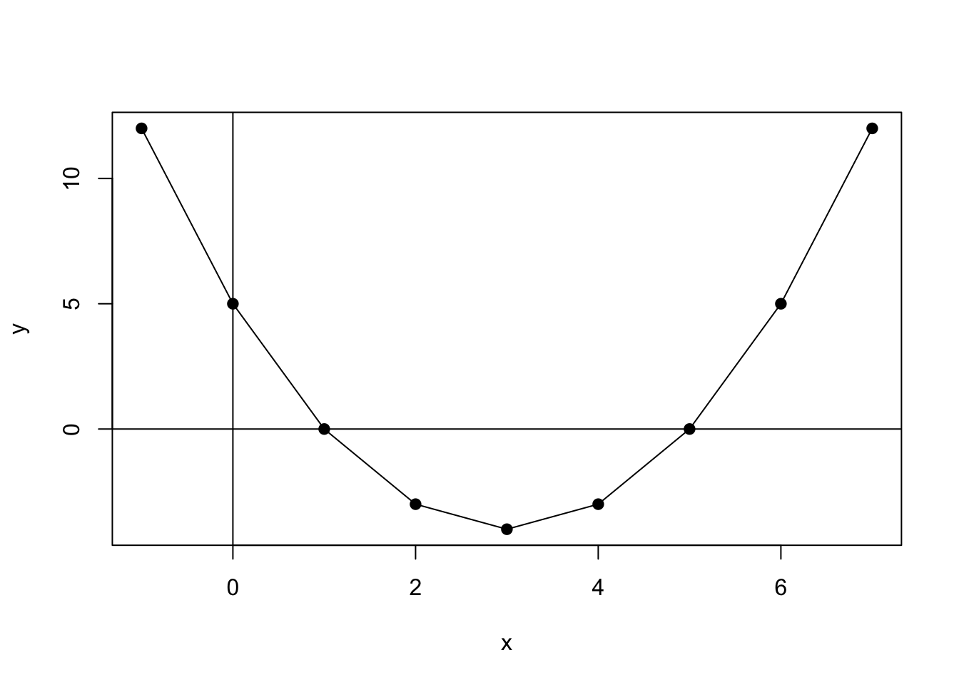
Figure 8.2: Plot of Function \(y=f(x)=x^2-6x+5\)
We can also use the derivative and R to calculate the slope for each value of \(X\).
## [1] -8 -6 -4 -2 0 2 4 6 8The values for \(X\), which are shown in Figure 8.2, range from -8 to +8 and return derivatives (slopes at a point) ranging from -25 to +25.
Rule 6: the Quotient Rule
Example: \[\begin{align*} f(x) &=\frac{x}{x^{2}+5} \\ f'(x)&=\frac{(x^{2}+5)(x)'-(x^{2}+5)'(x)}{(x^{2}+5)^{2}} \\ &=\frac{(x^{2}+5)-(2x)(x)}{(x^{2}+5)^{2}} \\ &= \frac{-x^{2}+5}{(x^{2}+5)^{2}} \end{align*}\]
Rule 7: the Chain Rule
Example: \[\begin{align*} f(x) &= (7x^{2}-2x+13)^{5} \\ f'(x)&=5(7x^{2}-2x+13)^{4}*(7x^{2}-2x+13)' \\ &=5(7x^{2}-2x+13)^{4}*(14x-2) \end{align*}\]
8.1.2 Critical Points
Our goal is to use derivatives to find the values of \(\hat{\alpha}\) and \(\hat{\beta}\) that minimize the sum of the squared error. To do this we need to find the minima of a function. The minima is the smallest value that a function takes, whereas the maxima is the largest value. To find the minima and maxima, the critical points are key. The critical point is where the derivative of the function is equal to \(0\), or \(f'(x)=0\). Note that this is equivalent to the slope being equal to \(0\).
Example: Finding the Critical Points
To find the critical point for the function
\(y=f(x)=(x^{2}-4x+5)\);
First find the derivative; \(f'(x)=2x-4\)
Set the derivative equal to \(0\); \(f'(x)=2x-4=0\)
Solve for \(x\); \(x=2\)
Substitute \(2\) for \(x\) into the function and solve for \(y\)
Thus, the critical point (there’s only one in this case) of the function is \((2,1)\)
Once a critical point is identified, the next step is to determine whether that point is a minima or a maxima. The most straightforward way to do this is to identify the x,y coordinates and plot. This can be done in R, as we will show using the function \(y=f(x)=(x^{2}-4x+5)\). The plot is shown in Figure 8.3.
## [1] -5 -4 -3 -2 -1 0 1 2 3 4 5## [1] 50 37 26 17 10 5 2 1 2 5 10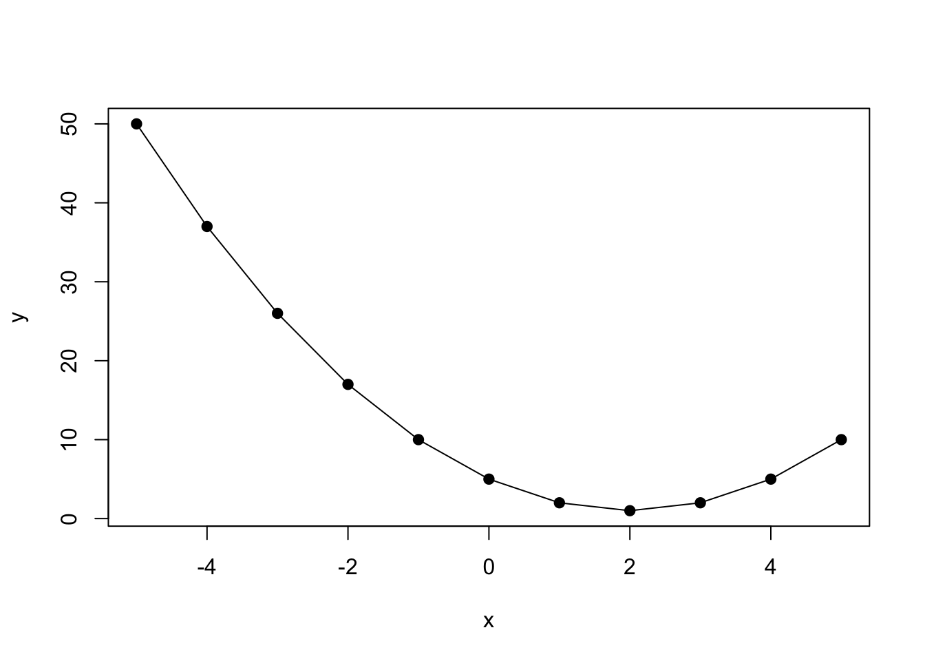
Figure 8.3: Identification of Critical Points
As can be seen, the critical point \((2,1)\) is a minima.
8.1.3 Partial Derivation
When an equation includes two variables, one can take a partial derivative with respect to only one variable, while the other variable is simply treated as a constant. This is particularly useful in our case, because the function \(\sum \epsilon^{2}\) has two variables – \(\hat{\alpha}\) and \(\hat{\beta}\).
Let’s take an example. For the function \(y=f(x,z)=x^{3}+4xz-5z^{2}\), we first take the derivative of \(x\) holding \(z\) constant.
\[\begin{align*} \frac{\partial y}{\partial x} &= \frac{\partial f(x,z)}{\partial x} \\ &= 3x^{2}+4z \end{align*}\]
Next we take the derivative of \(z\) holding \(x\) constant.
\[\begin{align*} \frac{\partial y}{\partial z} &= \frac{\partial f(x,z)}{\partial z} \\ &= 4x-10z \end{align*}\]
8.2 Deriving OLS Estimators
Now that we have developed some of the rules for differential calculus, we can see how OLS finds values of \(\hat{\alpha}\) and \(\hat{\beta}\) that minimize the sum of the squared error. In formal terms, let’s define the set, \(S(\hat{\alpha},\hat{\beta})\), as a pair of regression estimators that jointly determine the residual sum of squares given that: \(Y_{i}=\hat {Y}_{i}+\epsilon_{i}=\hat{\alpha}+\hat{\beta}X_{i}+\epsilon_{i}\). This function can be expressed:
\[\begin{equation*} S(\hat{\alpha},\hat{\beta})=\sum_{i=1}^{n} \epsilon^{2}_{i}=\sum (Y_{i}-\hat{Y_{i}})^{2}=\sum (Y_{i}-\hat{\alpha}-\hat{\beta} X_{i})^{2} \end{equation*}\]
First, we will derive \(\hat{\alpha}\).
8.2.1 OLS Derivation of \(\hat{\alpha}\)
Take the partial derivatives of \(S(\hat{\alpha},\hat{\beta})\) with-respect-to (w.r.t) \(\hat{\alpha}\) in order to determine the formulation of \(\hat{\alpha}\) that minimizes \(S(\hat{\alpha},\hat{\beta})\). Using the chain rule,
\[\begin{align*} \frac{\partial S(\hat{\alpha},\hat{\beta})}{\partial \hat{\alpha}} &= \sum 2(Y_{i}-\hat{\alpha}-\hat{\beta}X_{i})^{2-1}*(Y_{i}-\hat{\alpha}-\hat{\beta}X_{i})' \\ &= \sum 2(Y_{i}-\hat{\alpha}-\hat{\beta}X_{i})^{1}*(-1) \\ &= -2 \sum (Y_{i}-\hat{\alpha}-\hat{\beta}X_{i}) \\ &= -2 \sum Y_{i}+2n\hat{\alpha}+2\hat{\beta} \sum X_{i} \end{align*}\]
Next, set the derivative equal to \(0\).
\[\begin{equation*} \frac{\partial S(\hat{\alpha},\hat{\beta})}{\partial \hat{\alpha}} = -2 \sum Y_{i}+2n\hat{\alpha}+2\hat{\beta} \sum X_{i} = 0 \end{equation*}\]
Then, shift non-\(\hat{\alpha}\) terms to the other side of the equal sign:
\[\begin{equation*} 2n\hat{\alpha} = 2 \sum Y_{i}-2\hat{\beta} \sum X_{i} \end{equation*}\]
Finally, divide through by \(2n\): \[\begin{align*} \frac{2n\hat{\alpha}}{2n} &= \frac{2 \sum Y_{i}-2\hat{\beta} \sum X_{i}}{2n} \\ A &= \frac{\sum Y_{i}}{n}-\hat{\beta}*\frac{\sum X_{i}}{n} \\ &= \bar {Y}-\hat{\beta} \bar{X} \\ \end{align*}\]
\[\begin{equation} \therefore \hat{\alpha} = \bar {Y}-\hat{\beta} \bar{X} \tag{8.1} \end{equation}\]
8.2.2 OLS Derivation of \(\hat{\beta}\)
Having found \(\hat{\alpha}\), the next step is to derive \(\hat{\beta}\). This time we will take the partial derivative w.r.t \(\hat{\beta}\). As you will see, the steps are a little more involved for \(\hat{\beta}\) than they were for \(\hat{\alpha}\).
\[\begin{align*} \frac{\partial S(\hat{\alpha},\hat{\beta})}{\partial \hat{\beta}} &= \sum 2(Y_{i}-\hat{\alpha}-\hat{\beta}X_{i})^{2-1}*(Y_{i}-\hat{\alpha}-\hat{\beta}X_{i})' \\ &= \sum 2(Y_{i}-\hat{\alpha}-\hat{\beta}X_{i})^{1}*(-X_{i}) \\ &= 2 \sum (-X_{i}Y_{i}+\hat{\alpha}X_{i}+\hat{\beta}X^{2}_{i}) \\ &= -2 \sum X_{i}Y_{i}+2\hat{\alpha} \sum X_{i} + 2\hat{\beta} \sum X^{2}_{i} \end{align*}\]
Since we know that \(\hat{\alpha} = \bar {Y}-\hat{\beta} \bar{X}\), we can substitute \(\bar {Y}-\hat{\beta} \bar{X}\) for \(\hat{\alpha}\).
\[\begin{align*} \frac{\partial S(\hat{\alpha},\hat{\beta})}{\partial \hat{\beta}} &= -2 \sum X_{i}Y_{i}+2(\bar {Y}-\hat{\beta} \bar{X})\sum X_{i} + 2\hat{\beta} \sum X^{2}_{i} \\ &= -2 \sum X_{i}Y_{i}+2 \bar{Y} \sum X_{i}-2\hat{\beta} \bar{X} \sum X_{i} + 2\hat{\beta} \sum X^{2}_{i} \end{align*}\]
Next, we can substitute \(\frac{\sum Y_{i}}{n}\) for \(\bar{Y}\) and \(\frac{\sum X_{i}}{n}\) for \(\bar{X}\) and set it equal to \(0\).
\[\begin{equation*} \frac{\partial S(\hat{\alpha},\hat{\beta})}{\partial \hat{\beta}} = -2 \sum X_{i}Y_{i}+\frac{2\sum Y_{i} \sum X_{i}}{n}-\frac{2\hat{\beta}\sum X_{i} \sum X_{i}}{n}+ 2\hat{\beta} \sum X^{2}_{i} = 0 \end{equation*}\]
Then, multiply through by \(\frac{n}{2}\) and put all the \(\hat{\beta}\) terms on the same side.
\[\begin{align*} n\hat{\beta} \sum X^{2}_{i}-\hat{\beta}(\sum X_{i})^{2} &= n \sum X_{i}Y_{i}-\sum X_{i} \sum Y_{i} \\ \hat{\beta}(n \sum X^{2}_{i}-(\sum X_{i})^{2}) &= n \sum X_{i}Y_{i}-\sum X_{i} \sum Y_{i} \\ \therefore \hat{\beta} = \frac{n \sum X_{i}Y_{i}-\sum X_{i} \sum Y_{i}}{n\sum X^{2}_{i}-(\sum X_{i})^{2}} \end{align*}\]
The \(\hat{\beta}\) term can be rearranged such that:
\[\begin{equation} \hat{\beta}=\frac{\Sigma(X_{i}-\bar X)(Y_{i}-\bar Y)}{\Sigma(X_{i}-\bar X)^2} \tag{8.2} \end{equation}\]
Now remember what we are doing here: we used the partial derivatives for \(\sum \epsilon^{2}\) with respect to \(\hat{\alpha}\) and \(\hat{\beta}\) to find the values for \(\hat{\alpha}\) and \(\hat{\beta}\) that will give us the smallest value for \(\sum \epsilon^{2}\). Put differently, the formulas for \(\hat{\beta}\) and \(\hat{\alpha}\) allow the calculation of the error-minimizing slope (change in \(Y\) given a one unit change in \(X\)) and intercept (value for \(Y\) when \(X\) is zero) for any data set representing a bivariate, linear relationship. No other formulas will give us a line, using the same data, that will result in as small a squared-error. Therefore, OLS is referred to as the Best Linear Unbiased Estimator (BLUE).
8.2.3 Interpreting \(\hat{\beta}\) and \(\hat{\alpha}\)
In a regression equation, \(Y=\hat{\alpha}+\hat{\beta}X\), where \(\hat{\alpha}\) is shown in Equation (8.1) and \(\hat{\beta}\) is shown in Equation (8.2). Equation (8.2) shows that for each 1-unit increase in \(X\) you get \(\hat{\beta}\) units change in \(Y\). Equation (8.1) shows that when \(X\) is \(0\), \(Y\) is equal to \(\hat{\alpha}\). Note that in a regression model with no independent variables, \(\hat{\alpha}\) is simply the expected value (i.e., mean) of \(Y\).
The intuition behind these formulas can be shown by using R to calculate “by hand” the slope (\(\hat{\beta}\)) and intercept (\(\hat{\alpha}\)) coefficients. A theoretical simple regression model is structured as
follows:
\[\begin{equation*} Y_{i} = \alpha + \beta X_{i} + \epsilon_{i} \end{equation*}\]
- \(\alpha\) and \(\beta\) are constant terms
- \(\alpha\) is the intercept
- \(\beta\) is the slope
- \(X_{i}\) is a predictor of \(Y_{i}\)
- \(\epsilon\) is the error term
The model to be estimated is expressed as \(Y=\hat{\beta}+\hat{\beta}X+/epsilon\).
As noted, the goal is to calculate the intercept coefficient:
\[\begin{equation*} \hat{\alpha}=\bar Y-\hat{\beta}\bar X \end{equation*}\]
and the slope coefficient: \[\begin{equation*} \hat{\beta}=\frac{\Sigma(X_{i}-\bar X)(Y_{i}-\bar Y)}{\Sigma(X_{i}-\bar X)^2} \end{equation*}\]
Using R, this can be accomplished in a few steps. First create a vector of values for x and y (note that we chose these values arbitrarily for the purpose of this example).
## [1] 4 2 4 3 5 7 4 9## [1] 2 1 5 3 6 4 2 7Then, create objects for \(\bar {X}\) and \(\bar {Y}\):
## [1] 4.75## [1] 3.75Next, create objects for \((X-\bar X)\) and \((Y-\bar Y)\), the deviations of \(X\) and \(Y\) around their means:
## [1] -0.75 -2.75 -0.75 -1.75 0.25 2.25 -0.75 4.25## [1] -1.75 -2.75 1.25 -0.75 2.25 0.25 -1.75 3.25Then, calculate \(\hat{\beta}\):
\[\begin{equation*} \hat{\beta}=\frac{\Sigma(X_{i}-\bar X)(Y_{i}-\bar Y)}{\Sigma(X_{i}-\bar X)^2} \end{equation*}\]
## [1] 0.7183099Finally, calculate \(\hat{\alpha}\)
\[\begin{equation*} \hat{\alpha}=\bar Y-\hat{\beta}\bar X \end{equation*}\]
## [1] 0.3380282To see the relationship, we can produce a scatterplot of x and y and add our regression line, as shown in Figure 8.4. So, for each unit increase in \(x\), \(y\) increases by 0.7183099 and when \(x\) is \(0\), \(y\) is equal to 0.3380282.
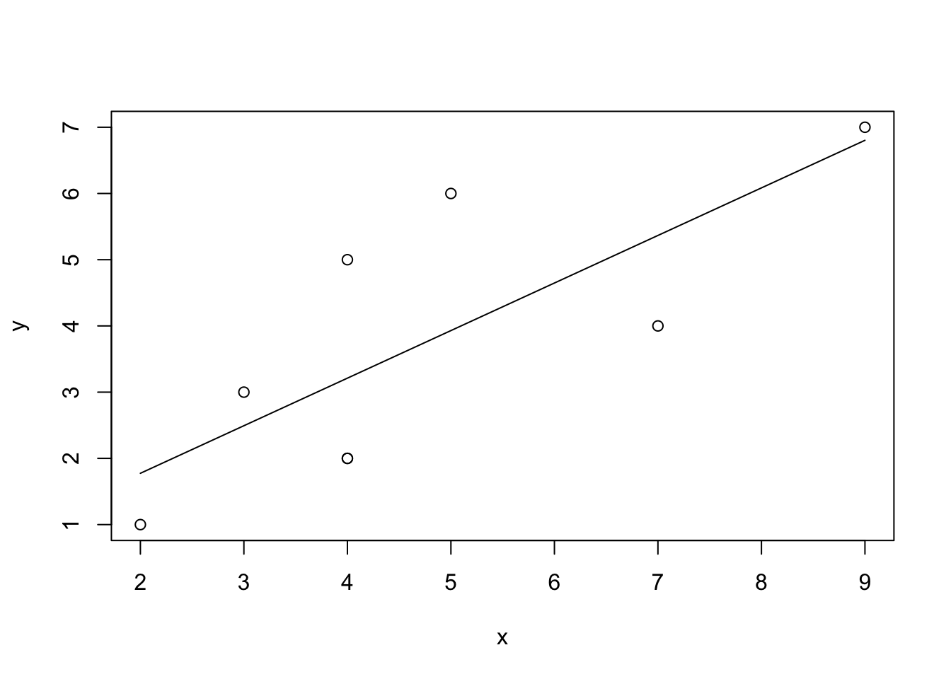
Figure 8.4: Simple Regression of \(x\) and \(y\)
## null device
##           1
8.3 Summary
Whoa! Think of what you’ve accomplished here: You learned enough calculus to find a minima for an equation with two variables, then applied that to the equation for the \(\sum \epsilon^{2}\). You derived the error minimizing values for \(\hat{\alpha}\) and \(\hat{\beta}\), then used those formulae in R to calculate ``by hand" the OLS regression for a small dataset.
Congratulate yourself – you deserve it!