Chapter 4 Machine Learning Model Classes
 14
Let us continue our penguin example introduced in 3.1. With our data pre-processed, the final step before fitting an ML model is to split our data.
14
Let us continue our penguin example introduced in 3.1. With our data pre-processed, the final step before fitting an ML model is to split our data.
4.1 Data Splitting
We need to split our pre-processed data into training and validation data sets. For our penguins example, we will call these data sets ml_penguin_train and ml_penguin_validate respectively.
We can use the createDataPartition function from the caret package to intelligently split the data into these two sets.
One benefit of using this function to split our data, compared to e.g. simply using the sample function, is that if our outcome variable is a factor (like species!) the random sampling employed by the createDataPartition function will occur within each class.
In other words, if we have a data set comprised roughly 50% Adelie penguin data, 20% Chinstrap data and 30% Gentoo data, the createDataPartition sampling will preserve this overall class distribution of 50/20/30.
Let’s take a look at how to use this function in RStudio:
set.seed(16505050)
train_index <- createDataPartition(ml_penguins_updated$species,
                                   p = .8, # here p designates the split - 80/20
                                   list = FALSE,
                                   times = 1) # times specifies how many splits to perform
Here we have split the training/validation data 80/20, via the argument p = 0.8. If we now take a quick look at our new object, we observe that:
head(train_index, n = 6)## Resample1
## [1,] 1
## [2,] 3
## [3,] 4
## [4,] 6
## [5,] 8
## [6,] 10Note that the observations 1, 3, 4, 6, 8 and 10 will now be assigned to the ml_penguin_train training data, while observations 2, 5 and 9 will be assigned to the ml_penguin_validate validation data.
The train_index object may contain the partition details, but we still need to assign our ml_penguin_train training data to specific training and validation objects in RStudio. To carry out these assignments we can use the following code:
ml_penguin_train <- ml_penguins_updated[train_index, ]
ml_penguin_validate  <- ml_penguins_updated[-train_index, ]
We are now ready to train our model!
4.2 Machine Learning Model Classes
Training a machine learning model using the caret package is deceptively simple in RStudio. We simply use the train function, specify our outcome variable and data set, and specify the model we would like to apply via the argument method = ....
However, there are over 200 available models in the caret package from which to choose15, and users can also specify their own models. Each model will have a different composition and different requirements, which we refer to as tuning parameters.
We can group different machine learning models into classes, and in this section we will provide a brief overview of some of the most popular classes of machine learning models, that will be suitable for supervised learning, following Thulin (2021).
The main classes of machine learning models are:
- Decision Trees
- Model Trees
- Random Forests
- Boosted Trees
- Linear Discriminant Analysis
- Support Vector Machines
- Nearest Neighbour Classifiers
We won’t go into all the mathematics behind these models. Rather, in the labs we will focus on the R code required to apply several of these to our data.
4.2.1 Tree Models
Tree models encompass several classes of machine learning model.
4.2.1.1 Decision Trees
The simplest type of tree model is a Decision Tree model.
The easiest way to describe a decision tree model is probably to show one - take a look at the result below, which uses our pre-processed ml_penguins_updated data from the example introduced in 3.1:
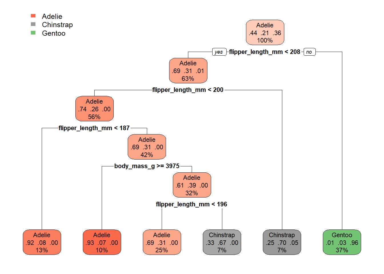
By starting at the top of the graph (the root), we can make decisions by following the branches until we arrive at a leaf node - i.e. Adelie, Chinstrap or Gentoo. The path from the root to the leaf represents the classification rules used in the model.
4.2.1.2 Model Trees
A model tree is like a decision tree, except that the regression model fitting process involved is more sophisticated.
Rather than using a single tree, we can use an ensemble method and combine multiple predictive models16. Random Forests and Boosted Trees are examples of ensemble tree models.
Random forest models combine multiple decision trees to achieve better results than any single decision tree considered could offer. Boosted tree models combine multiple decision trees, like random forest models, but use new trees to ‘boost’ (i.e. help) poorly performing trees.
4.2.2 Linear Models
A linear discriminant analysis (LDA) model is a type of linear model that uses Bayes’ theorem to classify new observations based on characteristics of the outcome variable classes.
4.2.3 Non-linear Models
A support vector machine (SVM) is a type of non-linear model that operates similarly to LDA models, with a focus on clearly separating outcome variable classes.
Nearest Neighbour Classifiers are another class of non-linear models, that assess distances between observations, grouping nearby observations together - a bit like k-means clustering.
4.3 Example - Gradient Boosting Machine model
To conclude this section, let’s go through an example application of the train function, using our filtered penguin data.
A gradient boosting machine is a type of boosted tree machine learning model.
To use this model, we specify method = gbm in the caret train function (you will need the gbm R package installed if you would like to replicate this - it may have been installed as part of the caret package installation).
Let’s take a look at this process now:
library(gbm)
set.seed(1650)
gbm_fit <- train(species ~ ., data = ml_penguin_train,
                 method = "gbm",
                 verbose = FALSE)
gbm_fit
## Stochastic Gradient Boosting
##
## 268 samples
## 4 predictor
## 3 classes: 'Adelie', 'Chinstrap', 'Gentoo'
##
## No pre-processing
## Resampling: Bootstrapped (25 reps)
## Summary of sample sizes: 268, 268, 268, 268, 268, 268, ...
## Resampling results across tuning parameters:
##
## interaction.depth n.trees Accuracy Kappa
## 1 50 0.8110186 0.6940950
## 1 100 0.8077852 0.6911365
## 1 150 0.7999774 0.6798165
## 2 50 0.8005603 0.6802749
## 2 100 0.7918955 0.6689067
## 2 150 0.7845712 0.6590680
## 3 50 0.7883501 0.6632650
## 3 100 0.7890195 0.6651849
## 3 150 0.7841261 0.6578865
##
## Tuning parameter 'shrinkage' was held constant at a value of 0.1
##
## Tuning parameter 'n.minobsinnode' was held constant at a value of 10
## Accuracy was used to select the optimal model using the largest value.
## The final values used for the model were n.trees = 50, interaction.depth =
## 1, shrinkage = 0.1 and n.minobsinnode = 10.Here we can see that the method has been carried out using different combinations of tuning parameters - which here include the number of training iterations to conduct (trees), the complexity of the trees (interaction.depth), and the adaptability or learning rate of the algorithm (shrinkage).
We are primarily interested in the Accuracy column in the output - this tells us the predictive accuracy of the model (based on the training data).
We can see that for 50 iterations, and an iteration complexity of 3, the gradient boosting machine achieves an accuracy of 97.81% using the training data.
We can use the plot function to visualise the results of this training process:
plot(gbm_fit)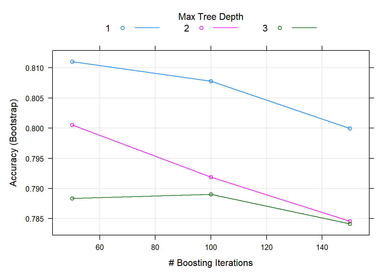
To use the top model to predict the species of penguin in our validation data, we can use the predict function used earlier (by default, the best performing model will be called from the gbm_fit object here):
ml_predictions <- predict(gbm_fit, newdata = ml_penguin_validate)
head(ml_predictions)
## [1] Adelie Adelie Adelie Adelie Adelie Adelie
## Levels: Adelie Chinstrap GentooNote that if you would like to see the probability associated with each result, you can include the argument type = "prob" within the predict function.
To compare these predictions with the actual species of penguin, we can use the following code - note that if the predicted and actual species match, we obtain a TRUE result, which counts as a 1, so that the output here denotes the number of correct predictions:
sum(ml_predictions == ml_penguin_validate$species)## [1] 53This is an excellent result, considering that our validation data consists of observations for 65 penguins.
We could extend this modelling process by tuning the parameters, but our results here are perfectly sufficient, and further work is beyond the scope of this subject.