Chapter 3 Supervised Machine Learning
using the caret R package
The caret (short for Classification And REgression Training) R package (Kuhn et al. 2021) contains a range of tools and models for conducting classification and regression machine learning in R. In fact, it offers over 200 different machine learning models from which to choose. Don’t worry, we don’t expect you to use them all!
In Computer Labs 9B - 11B we will use the caret R package to carry out supervised machine learning tasks in RStudio.
Recall that the typical process for a supervised ML task consists (with some simplifications) of 5 main steps:
- Define our aim
- Collect and pre-process data
- Split data into training and validation sets
- Use the training data to ‘train’ the ML model(s)
- Assess the predictive efficacy of the trained ML model(s) using the validation data
In the following sections we will demonstrate this process using the caret package and the familiar penguins data set from the palmerpenguins R package (Horst, Hill, and Gorman 2020).
Note: The details covered here should be transferable to other data sets.
3.1 Example Task: Predicting penguin species
Suppose we would like to use ML to predict the species of penguins in the Palmer archipelago, based on some of their other characteristics - namely their flipper_length_mm, body_mass_g and sex measurements (for this example we will ignore the other recorded variables in the penguins data set).
Therefore, we have a multi-class classification problem, with the feature variables flipper_length_mm, body_mass_g and sex, and the outcome variable species. Given we actually have recorded species observations already for all the penguins, our ML task can be categorised as a supervised learning task.
3.1.1 Preparations
To begin, we download, install and load the caret package in RStudio as follows:
install.packages("caret")
library(caret)
We also load the palmerpenguins package (which should already be installed).
library(palmerpenguins)Next, we create a new data set containing only our chosen feature and outcome variables (and also remove missing values):
ml_penguins <- na.omit(penguins[, c(1,5:7)])3.1.2 Data Visualisation
As we know by now, it is typically a good idea to visualise our data before conducting any analyses. Since we are already quite familiar with the penguins data set, we won’t spend too long on visualisations.
However, it is worthwhile to note that the caret package offers several options for visualising data, via the featurePlot function. We can use this function (with the argument plot = "pairs") to produce a scatter plot matrix of the different feature variables we are using, coloured by penguin species (as shown below).
Note: The featurePlot function’s plot argument can take several different options, such as density, box, and scatter - you might like to try these out.
featurePlot(x = ml_penguins[, -1], y = ml_penguins$species,
            plot = "pairs", auto.key = list(columns = 3))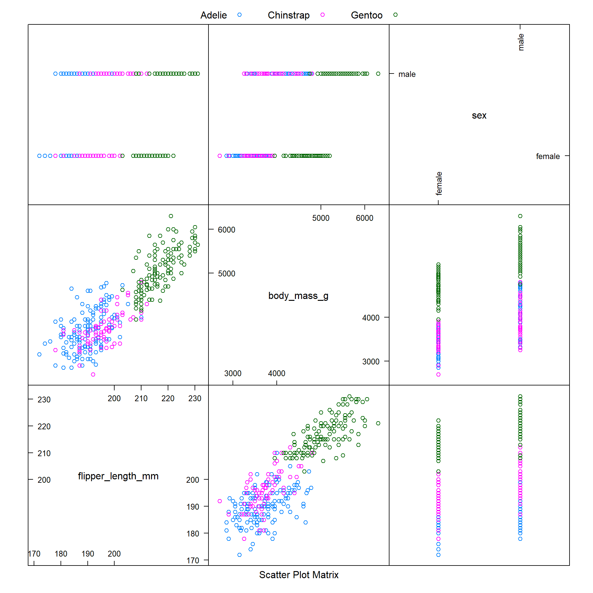
We observe that it is difficult to distinguish between Adelie and Chinstrap penguins when modelling body_mass_g against flipper_length_mm - these two species of penguins appear to have similar ranges of values for these variables.
Hopefully, as a result of training our machine learning model with our ml_penguins data, we will be able to accurately predict the species of these penguins.
3.2 Pre-Processing
The caret package contains several tools for pre-processing data, which makes our job easier.
3.2.1 Dummy Variables
One assumption made by the caret package is that all the feature variable data are numeric.
If our data contain one or more categorical feature variables, these will need to be converted to numeric variables before we train our ML model.
A dummy variable2 is a variable that only takes values of either 0 or 1, to indicate the absence or presence of a factor of interest, respectively. For example, if we had a dummy variable island = Dream, then this would equal 1 for all penguins living on Dream island, and 0 for penguins living on other islands.
Since our ml_penguins’ sex feature variable is categorical rather than numeric, we will have to convert it to a numeric variable.
We can use the dummyVars function from the caret package to reclassify the penguin sex recordings as dummy variables.
When converting feature variables via the dummayVars function, we need to follow a specific approach in RStudio, as detailed below:
# Load a package to help with the restructure of the data
library(tibble)

# Use the dummayVars function to create a full set of dummy variables for the ml_penguins data
dummy_penguins <- dummyVars(species ~ ., data = ml_penguins)

# Use the predict function to update our ml_penguins feature variables with sex dummy variables
ml_penguins_updated <- as_tibble(predict(dummy_penguins, newdata = ml_penguins))

# Prepend the outcome variable to our updated data set, otherwise it will be lost
ml_penguins_updated <- cbind(species = ml_penguins$species, ml_penguins_updated)
Note: We use the as_tibble function from the tibble package to restructure our data following the introduction of the dummyVars dummy variables. This is mainly because we would like to include the species variable with the labels Adelie, Chinstrap and Gentoo, rather than the numbers 1,2 and 3.
Note 2: Remember to always include the outcome variable when updating your data!
Now, instead of sex taking the values of female or male, this variable has been replaced by the dummy variables sex.female and sex.male, as shown below. Notice that in the first row, we have a value of 0 for sex.female and a value of 1 for sex.male - in other words, the data in the first row is for a male penguin.
| species | flipper_length_mm | body_mass_g | sex.female | sex.male |
|---|---|---|---|---|
| Adelie | 181 | 3750 | 0 | 1 |
| Adelie | 191 | 3700 | 0 | 1 |
| Gentoo | 217 | 4900 | 1 | 0 |
| Gentoo | 210 | 4700 | 1 | 0 |
| Chinstrap | 195 | 3600 | 0 | 1 |
| Chinstrap | 202 | 3400 | 1 | 0 |
3.2.2 Identifying samples exerting excessive influence
Before we begin training our machine learning model, we should also run some checks to ensure the quality of our data is high.
For instance, we should check our data to ensure that:
- Our data is balanced, with a large number of unique values for each feature variable
- There are no samples that might have an excessive influence on the model
- We do not have any highly correlated feature variables\(^\dagger\)
\(^\dagger\)Sometimes, a machine learning model will benefit from using training data which includes several highly correlated feature variables. Often however, correlated feature variables can be problematic.
3.2.3 Zero and Near-Zero Variance Feature Variables
If any feature variables have zero or near-zero variance, this can cause problems when we subsequently split our data into training and validation data sets.
We can use the nearZeroVar function from the caret package to check a and b on our checklist in 3.2.2.
One of the arguments of the nearZeroVar function is saveMetrics, which can be specified as either saveMetrics = F or saveMetrics = T.
- If we use
saveMetrics = F, a vector of the positions of the feature variables with zero or near-zero variance will be produced. - If we use
saveMetrics = T, a data frame with details about the variables will be produced.
Let’s consider both options, using our ml_penguins_updated data set.
saveMetrics = F option
nearZeroVar(ml_penguins_updated, saveMetrics = F)## integer(0)The output integer(0) means that none of the feature variables have been flagged as problematic, with respect to zero variance or near zero variance, which is encouraging. This means that none of the feature variables have only a single unique value.
saveMetrics = T option
nearZeroVar(ml_penguins_updated, saveMetrics = T)## freqRatio percentUnique zeroVar nzv
## species 1.226891 0.9009009 FALSE FALSE
## flipper_length_mm 1.235294 16.2162162 FALSE FALSE
## body_mass_g 1.200000 27.9279279 FALSE FALSE
## sex.female 1.018182 0.6006006 FALSE FALSE
## sex.male 1.018182 0.6006006 FALSE FALSEHere, we can see that as identified previously, none of the variables have zero or near zero variance (as shown in columns 3 and 4 of the output).
freqRatio: The freqRatio column computes the frequency of the most prevalent value recorded for that variable, divided by the frequency of the second most prevalent value. If we check this column, we see that all feature variables have a freqRatio value close to 1. This is good news, and means that we don’t have an unbalanced data set where one value is being recorded significantly more frequently than other values.
percentUnique: Finally, if we check the percentUnique column, we see the number of unique values recorded for each variable, divided by the total number of samples, and expressed as a percentage. If we only have a few unique values (i.e. the feature variable has near-zero variance) then the percentUnique value will be small. Therefore, higher values are considered better, but it is worth noting that as our data set increases in size, this percentage will naturally decrease.
Based on these results, we can see that none of the variables show concerning characteristics.
All the variables have
freqRatiovalues close to 1.The
species,sex.maleandsex.femalevariables have lowpercentUniquevalues, but this is to be expected for these types of variables (if they were continuous numeric variables, then this could be cause for concern). In other words, dummy variables often have lowpercentUniquevalues. This is normal and a lowpercentUniquevalue for a dummy feature variable is not by itself sufficient reason to remove the feature variable.
3.2.4 Cut-off Specifications
If we have certain pre-determined requirements for the freqRatio and percentUnique values, we can specify cut-off values using the arguments freqCut and uniqueCut respectively.
For example, suppose we considered feature variables with freqRatio scores higher than 1.23 and percentUnique scores lower than 20 to be exerting excessive influence. Then, we could use the following code to filter out such feature variables:
nearZeroVar(ml_penguins_updated, saveMetrics = T, freqCut = 1.23, uniqueCut = 20)## freqRatio percentUnique zeroVar nzv
## species 1.226891 0.9009009 FALSE FALSE
## flipper_length_mm 1.235294 16.2162162 FALSE TRUE
## body_mass_g 1.200000 27.9279279 FALSE FALSE
## sex.female 1.018182 0.6006006 FALSE FALSE
## sex.male 1.018182 0.6006006 FALSE FALSENotice how the output in the nzv column has changed compared to the initial output - now flipper_length_mm has an nzv value of TRUE, due to our arbitrary cut-off specifications.
3.2.4.1 Making conclusions based on cut-off values
In the event that a feature variable has both a high freqRatio value and a low percentUnique value, and both these values exceed the specified cut-offs, then it would be reasonable to remove this feature variable (assuming it is not a categorical variable).
If a feature variable has only one problematic value (e.g. a feature variable has a high freqRatio value that exceeds the specified cut-off, but also has a high percentUnique value which does not exceed the specified cut-off), then it is acceptable to retain this feature variable.