7 Natural Language Processing
Das Feld des NLP ist groß und selbst Bestandteil ganzer Vorlesungen, daher sind die folgenden Beispiele lediglich als kleiner Einblick zu verstehen. Hierbei soll lediglich der Umgang mit Texten im quantitativen Umfeld aufgezeigt werden. Als Beispiel dienen uns Finanznachrichten der Thomson Reuters Homepage, wobei alle dort verfügbaren Nachrichten von Unternehmen des Dow Jones Index gesammelt wurden.
rm(list = ls())

#load package for database connection
library(RSQLite)
library(dplyr)
library(tidytext)
library(tidytext)
library(tidyr)
library(tm)
library(topicmodels)
library(ggplot2)
library(data.table)


dt <- data.table(read.csv('Data/dji_reuters_crawl.csv'))

head(dt$date_string)
## [1] 2020-04-02 14:15:50 2020-04-01 02:31:16 2020-04-01 01:38:02
## [4] 2020-03-31 18:11:19 2020-03-31 16:20:49 2020-03-30 10:32:58
## 12651 Levels: 2017-03-20 04:04:06 2017-03-20 04:10:54 ... 2020-04-02 15:41:02## [1] NEW YORK (Reuters) - Goldman Sachs Group Inc (GS.N) Chief Executive David Solomon said Thursday Goldman is committing $250 million from its balance sheet to community development financial institutions so they can make loans to small businesses hurt by the coronavirus pandemic. Solomon also said that this own employees’ “jobs are safe” during this crisis. Reporting By Elizabeth Dilts Marshall
## [2] TOKYO (Reuters) - SoftBank Group Corp said on Wednesday it has appointed former Goldman Sachs banker Taiichi Hoshino as head of a new investment planning department, as the group increases oversight of its tech bets battered by volatile markets. Souring bets across its portfolio have left SoftBank selling down prime assets and holding back from making new investments. Hoshino is expected to bolster the investment team at a time when CEO Masayoshi Son has received criticism for his top-down investing approach. Ex-hedge fund manager Hoshino is the second SoftBank hire from a group at Japan Post Bank that was known as the “Seven Samurai” and tried a more aggressive investing strategy that has since been rolled back. The other is Katsunori Sago, also a Goldman alumnus, who became SoftBank’s chief strategy officer in 2018 and is seen as a possible successor to CEO Son. Hoshino is faced with an increasingly beleaguered portfolio, with satellite operator OneWeb, which embodied Son’s vision of a connected world, filing for Chapter 11 bankruptcy after failing to raise further funds. Shared-office operator WeWork is also facing growing pressure on its business model as workers stay home due to the coronavirus outbreak, and SoftBank is looking at walking away from a tender offer to employees and shareholders following its bailout of the firm. Reporting by Sam Nussey; Editing by Himani Sarkar and Tom Hogue
## [3] TOKYO, April 1 (Reuters) - SoftBank Group Corp said on Wednesday it has appointed former Goldman Sachs banker Taiichi Hoshino as head of a new investment planning department, as the group increases oversight of its tech bets battered by volatile markets. (Reporting by Sam Nussey; Editing by Himani Sarkar)
## [4] NEW YORK (Reuters) - Wall Street bank Goldman Sachs (GS.N) is offering employees 10 days of paid family leave to care for children or elderly parents who are at home during the coronavirus pandemic, according to a memo sent to staff on Tuesday that was seen by Reuters. Several banks have been extending extra paid time-off to employees, as the flu-like virus has shut down schools and forced many to stay at home. Reporting By Elizabeth Dilts Marshall; Editing by Chris Reese
## [5] (Reuters) - Goldman Sachs said on Tuesday the second-quarter U.S. economic decline would be much greater than it had previously forecast and unemployment would be higher, citing anecdotal evidence and “sky-high jobless claims numbers” resulting from the coronavirus pandemic. Goldman is now forecasting a real GDP sequential decline of 34% for the second quarter on an annualized basis, compared with its earlier estimate for a drop of 24%. It also cut its first-quarter target to a decline of 9% from its previous expectation for a 6% drop, according to chief economist Jan Hatzius. The firm now sees the unemployment rate rising to 15% by mid-year compared with its previous expectation for 9%. Jobless numbers show an even bigger collapse in output and labor market than Goldman previously expected, which Hatzius wrote “raises the specter of more adverse second-round effects on income and spending a bit further down the road.” The global spread of the novel coronavirus has pummeled economic expectations as many businesses have closed their doors, at least temporarily, as governments around the world ask people to stay at home to curtail further infections. U.S. President Donald Trump said on Monday that federal social distancing guidelines, including discouragement of gatherings larger than 10 people, might be toughened. On Sunday he announced an extension of current restrictions to April 30. Still, Goldman expects easing monetary and fiscal policy to help contain second-round effects on the economy and to add to growth down the road.” Goldman cited a much bigger-than-expected phase 3 U.S. fiscal package and forecast a phase 4 package for state fiscal aid, and the likelihood that the Fed would use the $454 billion addition to the Treasury’s Exchange Stabilization Fund aggressively to help credit flow to private-sector and municipal borrowers. Despite substantial uncertainty, Goldman said lockdowns and social distancing should sharply lower new infections in the next month. So a slower virus spread and adaptation by businesses and individuals “should set the stage for a gradual recovery in output starting in May/June.” As a result, it raised its expectation for a third-quarter GDP rebound to an annualized jump of 19% quarter-over-quarter, up from its previous target of 12% growth. It expects April GDP to be 13% below the January and February trend but that the drag then fades gradually by 10% each month in the services industry and by 12.5% in manufacturing and construction. In the United States, a Reuters tally shows coronavirus-related deaths reached 3,393 on Tuesday, ahead of China’s death toll. Reporting By Sinéad Carew, Editing by Franklin Paul and Bernadette Baum
## [6] LONDON (Reuters) - Goldman Sachs said on Monday it expects S&P 500 dividends to fall by 25% in 2020 as certain large dividend-paying industries are particularly vulnerable to the economic shock of the coronavirus outbreak. “The record high level of net leverage for the median S&P 500 stock coupled with the ongoing credit market stress means many firms are unlikely to borrow to fund their dividend,” Goldman said in a note. The U.S. investment bank said it expects a wave of dividends to be suspended, cut, and scrapped over the rest of the year. Reporting by Thyagaraju Adinarayan, Editing by Iain Withers
## 12637 Levels: ...7.1 Preprocessing
Bevor man die Texte verwenden kann, sollten sie bereinigt werden. Hierbei werden in der Regel Sonderzeichen, Großbuchstabeb, Zahlen und dergleichen entfernt. Zudem bietet es sich das tibble Paket mit seinen nützlichen Funktionen zu verwenden. Was wir hier nicht machen, jedoch erwähnenswert ist: Oft ist es sinnvoll nach sogenannten n-grams zu suchen und diese als ein Wort darzustellen. Gemeint damit sind getrennte Wörter, die jedoch zusammen etwas anderes bedeuten als getrennt. Ein Beispiel wäre olive oil.
#bring headlines to a tible data frame
#A tibble is a modern class of data frame within R, available in the dplyr and tibble packages,
#that has a convenient print method, will not convert strings to factors, and does not use row names.
#Tibbles are great for use with tidy tools.
text_df <- tibble(line = dt$X, document = dt$main_text)
head(text_df)
## # A tibble: 6 x 2
## line document
## <int> <fct>
## 1 0 NEW YORK (Reuters) - Goldman Sachs Group Inc (GS.N) Chief Executive Dav…
## 2 1 TOKYO (Reuters) - SoftBank Group Corp said on Wednesday it has appointe…
## 3 2 TOKYO, April 1 (Reuters) - SoftBank Group Corp said on Wednesday it has…
## 4 3 NEW YORK (Reuters) - Wall Street bank Goldman Sachs (GS.N) is offering …
## 5 4 (Reuters) - Goldman Sachs said on Tuesday the second-quarter U.S. econo…
## 6 5 LONDON (Reuters) - Goldman Sachs said on Monday it expects S&P 500 divi…#remove numbers and punctuation
text_tidy_df <- text_df %>%
mutate(document = gsub(x = document, pattern = '\\n{2}', replacement = ' ')) %>%
mutate(document = gsub(x = document, pattern = '[[:alnum:]]+\\@+[[:alnum:]]+[\\.]+[[:alnum:]]+|[[:alnum:]]+[\\.]+[[:alnum:]]+\\@+[[:alnum:]]+[\\.]+[[:alnum:]]+', replacement = '')) %>%
mutate(document = gsub(x = document, pattern = '[[:digit:]]|[[:punct:]]|http.*|www.*', replacement = '')) %>%
mutate(document = gsub(x = document, pattern = '([[:upper:]])', perl = TRUE, replacement = '\\L\\1'))
head(text_tidy_df)## # A tibble: 6 x 2
## line document
## <int> <chr>
## 1 0 new york reuters goldman sachs group inc gsn chief executive david sol…
## 2 1 tokyo reuters softbank group corp said on wednesday it has appointed f…
## 3 2 tokyo april reuters softbank group corp said on wednesday it has appo…
## 4 3 new york reuters wall street bank goldman sachs gsn is offering employ…
## 5 4 reuters goldman sachs said on tuesday the secondquarter us economic de…
## 6 5 london reuters goldman sachs said on monday it expects sp dividends t…#check for empty news and Na
out_empty <- apply(as.array(text_tidy_df$document), 1, nchar)
text_tidy_df <- text_tidy_df[out_empty != 0,]
out_na <- apply(as.array(text_tidy_df$document), 1, is.na)
text_tidy_df <- text_tidy_df[!out_na, ]
head(text_tidy_df)## # A tibble: 6 x 2
## line document
## <int> <chr>
## 1 0 new york reuters goldman sachs group inc gsn chief executive david sol…
## 2 1 tokyo reuters softbank group corp said on wednesday it has appointed f…
## 3 2 tokyo april reuters softbank group corp said on wednesday it has appo…
## 4 3 new york reuters wall street bank goldman sachs gsn is offering employ…
## 5 4 reuters goldman sachs said on tuesday the secondquarter us economic de…
## 6 5 london reuters goldman sachs said on monday it expects sp dividends t…## # A tibble: 6 x 2
## line word
## <int> <chr>
## 1 0 new
## 2 0 york
## 3 0 reuters
## 4 0 goldman
## 5 0 sachs
## 6 0 groupZunächst sollte man sich einen kleinen Überblick verschaffen. Je achdem, welche Methodik man später verwenden möchte, kann es sinnvoll sein, sogenannte Stop Words zu entfernen. Hierbei handelt es sich um Wörter, die häufig in allen Nachrichten vorkommen und daher keine Differenzierungsmöglichkeit mit sich bringen.
############################################################
#Counting Words
############################################################
#let us take a look at the most used words in our dataset
text_tidy_df %>%
count(word, sort = TRUE)## # A tibble: 51,021 x 2
## word n
## <chr> <int>
## 1 the 172050
## 2 to 97707
## 3 in 83170
## 4 of 77691
## 5 and 77580
## 6 a 70694
## 7 on 40045
## 8 by 40005
## 9 for 36865
## 10 said 36326
## # … with 51,011 more rows#maybe we should remove stop words first
text_tidy_df <- text_tidy_df %>%
anti_join(stop_words, by = 'word')
#let us take a look at the most used words in our dataset
text_tidy_df %>%
count(word, sort = TRUE)## # A tibble: 50,383 x 2
## word n
## <chr> <int>
## 1 reuters 16840
## 2 percent 15223
## 3 company 13236
## 4 billion 13112
## 5 reporting 10926
## 6 apple 10387
## 7 boeing 10275
## 8 editing 9412
## 9 million 7561
## 10 sales 5633
## # … with 50,373 more rows7.2 Sentiment
Es existieren verschiedene Sentiment Wörterbücher, die zum Großteil auf die subjektive Einteilung eines oder mehrerer Individuen zurück gehen. Für den Finanzkontext ist es meist sinnvoll, die für diesen Bereich definierten Wörterbücher zu verwenden, da Wörter existieren, die im Finanzkontext eine andere Bedeutung haben, als im allgemeinen Sprachgebrauch. Beispiele wären Bär und Bulle bzw. bear und bull um Marktphasen zu beschreiben. Zum Ende dieses Codeblocks halten wir für jede Nachricht fest, wie oft Wörter aus den sechs von Loughran und McDonald definierten Wörterbüchern vorgekommen sind. Dies kann man als quantitative Zusammenfassung ansehen, die für die Verwendung in einem quantitativen Modell geeignet wäre.
############################################################
#Counting Words with sentiment
############################################################
#let us take a look to the most negative and positive words in out dataset
#if we use the bing sentiment word list
text_tidy_df %>%
inner_join(get_sentiments('bing')) %>%
count(word, sort = TRUE, sentiment) %>%
group_split(sentiment)## [[1]]
## # A tibble: 2,078 x 3
## word sentiment n
## <chr> <chr> <int>
## 1 fell negative 2522
## 2 cancer negative 1442
## 3 rival negative 1363
## 4 concerns negative 1259
## 5 issues negative 1097
## 6 cloud negative 1029
## 7 crashes negative 999
## 8 risk negative 987
## 9 crash negative 981
## 10 crude negative 926
## # … with 2,068 more rows
##
## [[2]]
## # A tibble: 1,037 x 3
## word sentiment n
## <chr> <chr> <int>
## 1 trump positive 1603
## 2 strong positive 1462
## 3 top positive 1447
## 4 approval positive 1101
## 5 support positive 1096
## 6 led positive 976
## 7 helped positive 946
## 8 boost positive 918
## 9 worth positive 901
## 10 lead positive 832
## # … with 1,027 more rows
##
## attr(,"ptype")
## # A tibble: 0 x 3
## # … with 3 variables: word <chr>, sentiment <chr>, n <int>#we take a look at word counts for six financial states
#if we use the financial sentiment data set by Loughran and McDonald (2011)
text_tidy_df %>%
inner_join(get_sentiments('loughran')) %>%
count(word, sort = TRUE, sentiment) %>%
group_by(sentiment) %>%
top_n(5, n) %>%
ungroup() %>%
mutate(word = reorder(word, n)) %>%
ggplot(aes(word, n)) +
geom_col() +
coord_flip() +
facet_wrap(~ sentiment, scales = "free") +
ylab("Frequency of this word in the headlines")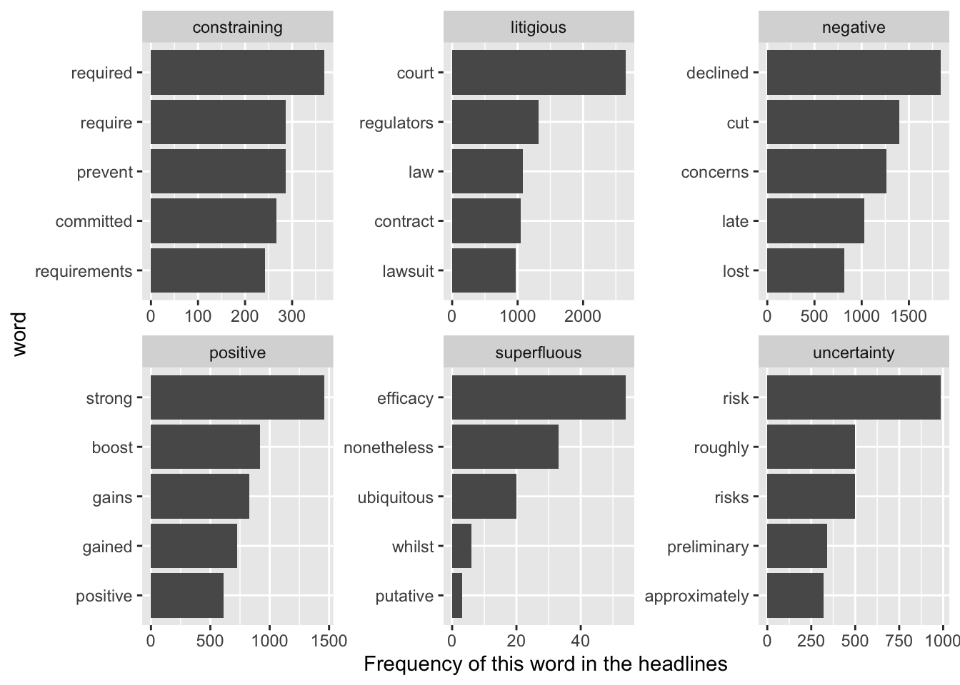
#and we can take a look at the frequency of these sentiment words per headline
loughran_mac_word_vecs <- text_tidy_df %>%
left_join(get_sentiments('loughran')) %>%
count(sentiment, line) %>%
arrange(line) %>%
spread(sentiment, n, fill = 0)
dt_out <- text_df %>%
inner_join(loughran_mac_word_vecs, by = 'line')
dt_out #<- data.table(dt_out)## # A tibble: 13,000 x 9
## line document constraining litigious negative positive superfluous
## <int> <fct> <dbl> <dbl> <dbl> <dbl> <dbl>
## 1 0 NEW YOR… 9 37 96 27 0
## 2 1 TOKYO (… 7 30 154 39 0
## 3 2 TOKYO, … 13 48 141 24 0
## 4 3 NEW YOR… 5 11 123 46 3
## 5 4 (Reuter… 11 60 136 22 0
## 6 5 LONDON … 11 31 102 38 1
## 7 6 BRASILI… 12 20 115 35 0
## 8 7 March 2… 12 54 129 26 0
## 9 8 BEIJING… 15 28 82 29 0
## 10 9 March 2… 22 19 143 40 1
## # … with 12,990 more rows, and 2 more variables: uncertainty <dbl>,
## # `<NA>` <dbl>7.3 LDA - Topicmodellierung
Als Alternative wird im folgenden Codeblock gezeigt, wie man mittels der Topicmodellierung Nachrichtenspezifische Vektoren (hier immer die Spalte) erzeugen kann. Beispielhaft werden hier vier Topics festgelegt, dies ist an dieser Stelle eine willkürliche Wahl.
############################################################
#LDA
############################################################
#remove numbers and punctuation
text_tidy_df <- text_df %>%
mutate(document = gsub(x = document, pattern = '\\n{2}', replacement = ' ')) %>%
mutate(document = gsub(x = document, pattern = '[[:alnum:]]+\\@+[[:alnum:]]+[\\.]+[[:alnum:]]+|[[:alnum:]]+[\\.]+[[:alnum:]]+\\@+[[:alnum:]]+[\\.]+[[:alnum:]]+', replacement = '')) %>%
mutate(document = gsub(x = document, pattern = '[[:digit:]]|[[:punct:]]|http.*|www.*', replacement = '')) %>%
mutate(document = gsub(x = document, pattern = '([[:upper:]])', perl = TRUE, replacement = '\\L\\1'))
#check for empty news and Na
out_empty <- apply(as.array(text_tidy_df$document), 1, nchar)
text_tidy_df <- text_tidy_df[out_empty != 0,]
out_na <- apply(as.array(text_tidy_df$document), 1, is.na)
text_tidy_df <- text_tidy_df[!out_na, ]
#unnest single words, remove stop words, prepare for document term matrix
line_words <- text_tidy_df %>%
unnest_tokens(word, document) %>%
anti_join(stop_words) %>%
count(line, word, sort = TRUE) %>%
arrange(line)
line_words## # A tibble: 1,059,498 x 3
## line word n
## <int> <chr> <int>
## 1 0 reuters 31
## 2 0 coronavirus 26
## 3 0 company 25
## 4 0 million 18
## 5 0 united 17
## 6 0 editing 16
## 7 0 reporting 16
## 8 0 march 15
## 9 0 apple 12
## 10 0 business 12
## # … with 1,059,488 more rows#Topic analysis
#First, we need to bring the tidy document into a differnt form, before we apply topic analysis methods
document_matrix <- cast_dfm(line_words, line, word, n)
#fit a lda model with two topics
lda_model <- LDA(document_matrix, k = 4, control = list(seed = 1234))
#probability for each word to belong to topic
lda_topics <- tidy(lda_model, matrix = 'beta')
#visualize probabilities for top ten words with highest probabilities for each categorie
lda_top_terms <- lda_topics %>%
group_by(topic) %>%
top_n(10, beta) %>%
ungroup() %>%
arrange(topic, -beta)
lda_top_terms %>%
mutate(term = reorder_within(term, beta, topic)) %>%
ggplot(aes(term, beta, fill = factor(topic))) +
geom_col(show.legend = FALSE) +
facet_wrap(~ topic, scales = "free") +
coord_flip() +
scale_x_reordered()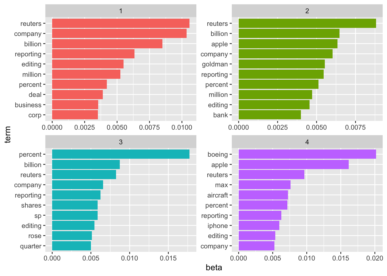
lda_documents <- tidy(lda_model, matrix = "gamma")
lda_documents <- lda_documents %>%
spread(topic, gamma) %>%
arrange(as.numeric(document))
names(lda_documents)[1] <- 'line'
lda_documents$line <- as.integer(lda_documents$line)
dt_out <- text_df %>%
inner_join(lda_documents, by = 'line')
dt_out #<- data.table(dt_out)## # A tibble: 13,000 x 6
## line document `1` `2` `3` `4`
## <int> <fct> <dbl> <dbl> <dbl> <dbl>
## 1 0 NEW YORK (Reuters) - Goldman Sachs Group … 0.355 9.40e-2 0.551 3.15e-5
## 2 1 TOKYO (Reuters) - SoftBank Group Corp sai… 0.229 2.81e-5 0.771 2.81e-5
## 3 2 TOKYO, April 1 (Reuters) - SoftBank Group… 0.367 2.96e-5 0.633 2.96e-5
## 4 3 NEW YORK (Reuters) - Wall Street bank Gol… 0.315 2.86e-5 0.685 2.86e-5
## 5 4 (Reuters) - Goldman Sachs said on Tuesday… 0.449 3.21e-5 0.551 3.21e-5
## 6 5 LONDON (Reuters) - Goldman Sachs said on … 0.658 2.81e-5 0.342 2.81e-5
## 7 6 BRASILIA (Reuters) - Latin America’s econ… 0.365 2.62e-5 0.635 2.62e-5
## 8 7 March 27 (Reuters) - Clicks Group Ltd: * … 0.715 2.55e-5 0.249 3.61e-2
## 9 8 BEIJING/HONG KONG (Reuters) - Goldman Sac… 0.282 5.60e-2 0.555 1.08e-1
## 10 9 March 26 (Reuters) - Goldman Sachs expect… 0.220 2.18e-5 0.778 2.41e-3
## # … with 12,990 more rows## # A tibble: 6 x 6
## line document `1` `2` `3` `4`
## <int> <fct> <dbl> <dbl> <dbl> <dbl>
## 1 2292 "(Reuters) - Boeing Co and Airbus Group … 0.0680 5.86e-4 5.86e-4 0.931
## 2 2293 "(Adds Boeing statement) March 24 (Reute… 0.0647 5.28e-4 5.28e-4 0.934
## 3 2294 "March 24 (Reuters) - Boeing Co and Airb… 0.000619 6.19e-4 6.19e-4 0.998
## 4 2295 "SEATTLE (Reuters) - A U.S. tax overhaul… 0.000210 5.76e-2 1.28e-1 0.814
## 5 2296 "March 23 (Reuters) - Boeing * Boeing sa… 0.00497 4.97e-3 4.97e-3 0.985
## 6 2297 "March 21 (Reuters) - Boc Aviation Ltd: … 0.00251 5.73e-1 2.51e-3 0.4227.4 Word Embedding
Als letztes möchte ich Ihnen lediglich noch zeigen, wie word embeddings in R geschätzt werden können. Hierfür suchen wir uns ein prominentes Beispiel - Word2Vec - heraus. Word2Vec wird normalerweise über den sogenannten Skip-Gram Algorithmus geschätzt, bei dem die Vektoren der Wörter so geschätzt werden, dass die Wahrscheinlichkeit eines gemeinsamen Auftretens maximiert wird. Kommt es beispielsweise oft zu dem Satz “High gains after bull market”, so wird das Modell erkennen, dass “gain” und “bull” oft zusammen auftreten und die Vektoren der beiden Wörter werden ähnlich sein. In R kann dieses Modell mittels eines Pakets geschätzt werden.
## # A tibble: 6 x 2
##    line document
##   <int> <fct>
## 1     0 NEW YORK (Reuters) - Goldman Sachs Group Inc (GS.N) Chief Executive Dav…
## 2     1 TOKYO (Reuters) - SoftBank Group Corp said on Wednesday it has appointe…
## 3     2 TOKYO, April 1 (Reuters) - SoftBank Group Corp said on Wednesday it has…
## 4     3 NEW YORK (Reuters) - Wall Street bank Goldman Sachs (GS.N) is offering …
## 5     4 (Reuters) - Goldman Sachs said on Tuesday the second-quarter U.S. econo…
## 6     5 LONDON (Reuters) - Goldman Sachs said on Monday it expects S&P 500 divi…
#remove numbers and punctuation
text_tidy_df <- text_df %>%
mutate(document = gsub(x = document, pattern = '\\n{2}', replacement = ' ')) %>%
mutate(document = gsub(x = document, pattern = '[[:alnum:]]+\\@+[[:alnum:]]+[\\.]+[[:alnum:]]+|[[:alnum:]]+[\\.]+[[:alnum:]]+\\@+[[:alnum:]]+[\\.]+[[:alnum:]]+', replacement = '')) %>%
mutate(document = gsub(x = document, pattern = '[[:digit:]]|[[:punct:]]|http.*|www.*', replacement = '')) %>%
mutate(document = gsub(x = document, pattern = '([[:upper:]])', perl = TRUE, replacement = '\\L\\1'))
head(text_tidy_df)## # A tibble: 6 x 2
## line document
## <int> <chr>
## 1 0 new york reuters goldman sachs group inc gsn chief executive david sol…
## 2 1 tokyo reuters softbank group corp said on wednesday it has appointed f…
## 3 2 tokyo april reuters softbank group corp said on wednesday it has appo…
## 4 3 new york reuters wall street bank goldman sachs gsn is offering employ…
## 5 4 reuters goldman sachs said on tuesday the secondquarter us economic de…
## 6 5 london reuters goldman sachs said on monday it expects sp dividends t…#one news per list entry
all_news <- as.list(text_tidy_df$document)
#write each news to a single txt-file
for(i in 1:dim(text_tidy_df)[1]){
write.table(all_news[[i]], file = paste('w2v_dji/w2v_dji_news_', i, '.txt', sep = ''), quote = FALSE, row.names = FALSE, col.names = FALSE)
}
#require necessary word2vec models
if (!require(wordVectors)) {
if (!(require(devtools))) {
install.packages("devtools")
}
devtools::install_github("bmschmidt/wordVectors")
}
library(wordVectors)
library(magrittr)
#preprocessing
prep_word2vec(origin="w2v_dji",destination="w2v_dji.txt",lowercase=T,bundle_ngrams=2)## Starting training using file w2v_dji.txt
## Words processed: 100K Vocab size: 52K
Words processed: 200K Vocab size: 90K
Words processed: 300K Vocab size: 121K
Words processed: 400K Vocab size: 146K
Words processed: 500K Vocab size: 169K
Words processed: 600K Vocab size: 188K
Words processed: 700K Vocab size: 212K
Words processed: 800K Vocab size: 234K
Words processed: 900K Vocab size: 257K
Words processed: 1000K Vocab size: 286K
Words processed: 1100K Vocab size: 314K
Words processed: 1200K Vocab size: 339K
Words processed: 1300K Vocab size: 363K
Words processed: 1400K Vocab size: 388K
Words processed: 1500K Vocab size: 411K
Words processed: 1600K Vocab size: 433K
Words processed: 1700K Vocab size: 453K
Words processed: 1800K Vocab size: 472K
Words processed: 1900K Vocab size: 491K
Words processed: 2000K Vocab size: 514K
Words processed: 2100K Vocab size: 536K
Words processed: 2200K Vocab size: 555K
Words processed: 2300K Vocab size: 576K
Words processed: 2400K Vocab size: 596K
Words processed: 2500K Vocab size: 615K
Words processed: 2600K Vocab size: 634K
Words processed: 2700K Vocab size: 650K
Words processed: 2800K Vocab size: 666K
Words processed: 2900K Vocab size: 681K
Words processed: 3000K Vocab size: 698K
Words processed: 3100K Vocab size: 714K
Words processed: 3200K Vocab size: 731K
Words processed: 3300K Vocab size: 749K
## Vocab size (unigrams + bigrams): 438141
## Words in train file: 3363228
## Words written: 100K
Words written: 200K
Words written: 300K
Words written: 400K
Words written: 500K
Words written: 600K
Words written: 700K
Words written: 800K
Words written: 900K
Words written: 1000K
Words written: 1100K
Words written: 1200K
Words written: 1300K
Words written: 1400K
Words written: 1500K
Words written: 1600K
Words written: 1700K
Words written: 1800K
Words written: 1900K
Words written: 2000K
Words written: 2100K
Words written: 2200K
Words written: 2300K
Words written: 2400K
Words written: 2500K
Words written: 2600K
Words written: 2700K
Words written: 2800K
Words written: 2900K
Words written: 3000K
Words written: 3100K
Words written: 3200K
Words written: 3300K#training...can take a while
vec_length <- 100
if (!file.exists("w2v_dji.txt.bin")){
model <- train_word2vec("w2v_dji.txt","w2v_dji.txt.bin", vectors = vec_length, threads = 4) }else{
model <- read.vectors("w2v_dji.txt.bin")
}##
|
| | 0%
|
| | 1%
|
|= | 1%
|
|= | 2%
|
|== | 2%
|
|== | 3%
|
|== | 4%
|
|=== | 4%
|
|=== | 5%
|
|==== | 5%
|
|==== | 6%
|
|===== | 6%
|
|===== | 7%
|
|===== | 8%
|
|====== | 8%
|
|====== | 9%
|
|======= | 9%
|
|======= | 10%
|
|======= | 11%
|
|======== | 11%
|
|======== | 12%
|
|========= | 12%
|
|========= | 13%
|
|========= | 14%
|
|========== | 14%
|
|========== | 15%
|
|=========== | 15%
|
|=========== | 16%
|
|============ | 16%
|
|============ | 17%
|
|============ | 18%
|
|============= | 18%
|
|============= | 19%
|
|============== | 19%
|
|============== | 20%
|
|============== | 21%
|
|=============== | 21%
|
|=============== | 22%
|
|================ | 22%
|
|================ | 23%
|
|================ | 24%
|
|================= | 24%
|
|================= | 25%
|
|================== | 25%
|
|================== | 26%
|
|=================== | 26%
|
|=================== | 27%
|
|=================== | 28%
|
|==================== | 28%
|
|==================== | 29%
|
|===================== | 29%
|
|===================== | 30%
|
|===================== | 31%
|
|====================== | 31%
|
|====================== | 32%
|
|======================= | 32%
|
|======================= | 33%
|
|======================= | 34%
|
|======================== | 34%
|
|======================== | 35%
|
|========================= | 35%
|
|========================= | 36%
|
|========================== | 36%
|
|========================== | 37%
|
|========================== | 38%
|
|=========================== | 38%
|
|=========================== | 39%
|
|============================ | 39%
|
|============================ | 40%
|
|============================ | 41%
|
|============================= | 41%
|
|============================= | 42%
|
|============================== | 42%
|
|============================== | 43%
|
|============================== | 44%
|
|=============================== | 44%
|
|=============================== | 45%
|
|================================ | 45%
|
|================================ | 46%
|
|================================= | 46%
|
|================================= | 47%
|
|================================= | 48%
|
|================================== | 48%
|
|================================== | 49%
|
|=================================== | 49%
|
|=================================== | 50%
|
|=================================== | 51%
|
|==================================== | 51%
|
|==================================== | 52%
|
|===================================== | 52%
|
|===================================== | 53%
|
|===================================== | 54%
|
|====================================== | 54%
|
|====================================== | 55%
|
|======================================= | 55%
|
|======================================= | 56%
|
|======================================== | 56%
|
|======================================== | 57%
|
|======================================== | 58%
|
|========================================= | 58%
|
|========================================= | 59%
|
|========================================== | 59%
|
|========================================== | 60%
|
|========================================== | 61%
|
|=========================================== | 61%
|
|=========================================== | 62%
|
|============================================ | 62%
|
|============================================ | 63%
|
|============================================ | 64%
|
|============================================= | 64%
|
|============================================= | 65%
|
|============================================== | 65%
|
|============================================== | 66%
|
|=============================================== | 66%
|
|=============================================== | 67%
|
|=============================================== | 68%
|
|================================================ | 68%
|
|================================================ | 69%
|
|================================================= | 69%
|
|================================================= | 70%
|
|================================================= | 71%
|
|================================================== | 71%
|
|================================================== | 72%
|
|=================================================== | 72%
|
|=================================================== | 73%
|
|=================================================== | 74%
|
|==================================================== | 74%
|
|==================================================== | 75%
|
|===================================================== | 75%
|
|===================================================== | 76%
|
|====================================================== | 76%
|
|====================================================== | 77%
|
|====================================================== | 78%
|
|======================================================= | 78%
|
|======================================================= | 79%
|
|======================================================== | 79%
|
|======================================================== | 80%
|
|======================================================== | 81%
|
|========================================================= | 81%
|
|========================================================= | 82%
|
|========================================================== | 82%
|
|========================================================== | 83%
|
|========================================================== | 84%
|
|=========================================================== | 84%
|
|=========================================================== | 85%
|
|============================================================ | 85%
|
|============================================================ | 86%
|
|============================================================= | 86%
|
|============================================================= | 87%
|
|============================================================= | 88%
|
|============================================================== | 88%
|
|============================================================== | 89%
|
|=============================================================== | 89%
|
|=============================================================== | 90%
|
|=============================================================== | 91%
|
|================================================================ | 91%
|
|================================================================ | 92%
|
|================================================================= | 92%
|
|================================================================= | 93%
|
|================================================================= | 94%
|
|================================================================== | 94%
|
|================================================================== | 95%
|
|=================================================================== | 95%
|
|=================================================================== | 96%
|
|==================================================================== | 96%
|
|==================================================================== | 97%
|
|==================================================================== | 98%
|
|===================================================================== | 98%
|
|===================================================================== | 99%
|
|======================================================================| 99%
|
|======================================================================| 100%## word similarity to "trump"
## 1 trump 1.0000000
## 2 president_donald 0.8941386
## 3 trumps 0.8341182
## 4 impeachment 0.7471516
## 5 white_house 0.7392360
## 6 progrowth_policies 0.7087279
## 7 trumps_comments 0.7082881
## 8 trump_took 0.7062243
## 9 rollback 0.6951887
## 10 flaming_out 0.6943600## [,1] [,2] [,3] [,4] [,5] [,6]
## [1,] -0.1509639 -0.5083545 0.02464562 -0.1149522 -0.2041776 -0.655957
## [,7] [,8] [,9] [,10] [,11] [,12]
## [1,] -0.6815168 -0.2204803 -0.07469373 0.2629436 -0.4867288 0.05361294
## [,13] [,14] [,15] [,16] [,17] [,18] [,19]
## [1,] -0.06677222 0.4039207 -0.5347745 0.6471485 0.03668177 -0.2361454 0.8404019
## [,20] [,21] [,22] [,23] [,24] [,25]
## [1,] 0.1680952 -0.001276304 0.6335668 0.5151724 -0.02500073 -0.03312694
## [,26] [,27] [,28] [,29] [,30] [,31]
## [1,] 0.1175454 0.3816812 -0.6069105 0.05233769 -0.06143506 0.08629163
## [,32] [,33] [,34] [,35] [,36] [,37] [,38]
## [1,] -0.1533257 0.1445092 -0.3223245 -0.4147433 -0.6708255 -0.359766 0.07986429
## [,39] [,40] [,41] [,42] [,43] [,44]
## [1,] -0.1797991 0.03839701 -0.2493985 0.2746376 -0.01088239 0.4848867
## [,45] [,46] [,47] [,48] [,49] [,50] [,51]
## [1,] 0.01983293 0.3012545 0.3496974 -0.01087733 0.0176043 0.4188663 0.1015002
## [,52] [,53] [,54] [,55] [,56] [,57]
## [1,] 0.04736793 0.4634666 -0.00458773 -0.2897104 -0.2453205 0.08664793
## [,58] [,59] [,60] [,61] [,62] [,63] [,64]
## [1,] -0.09907734 0.2692068 -0.2334383 -0.039895 0.1668558 0.3255708 -0.2124194
## [,65] [,66] [,67] [,68] [,69] [,70]
## [1,] 0.07076212 0.7358175 0.06938152 -0.1429023 0.1490907 -0.9262408
## [,71] [,72] [,73] [,74] [,75] [,76] [,77]
## [1,] -0.08199216 0.134671 -0.03161394 0.3348458 0.1713883 0.2294427 -0.06940857
## [,78] [,79] [,80] [,81] [,82] [,83] [,84]
## [1,] -0.707267 -0.03353878 0.4885126 -0.2517583 -0.1800412 0.0701581 -0.1242435
## [,85] [,86] [,87] [,88] [,89] [,90]
## [1,] -0.07970908 0.238446 0.05980043 -0.3515217 0.005761489 -0.3772532
## [,91] [,92] [,93] [,94] [,95] [,96] [,97]
## [1,] -0.3264284 1.066325 -0.627253 -0.4002535 0.1210985 0.2307914 0.1099931
## [,98] [,99] [,100]
## [1,] 0.2137776 -0.2579398 0.04234225#words can be put in distinct classes like for LDA, here for example by k-means algorithm
set.seed(10)
centers = 150
clustering = kmeans(model,centers=centers,iter.max = 40)
sapply(sample(1:centers,10),function(n) {
names(clustering$cluster[clustering$cluster==n][1:10])
})## [,1] [,2] [,3]
## [1,] "did_not" "coverage" "reporting_by"
## [2,] "comment" "further_company" "editing_by"
## [3,] "declined_to" "source_text" "in_bengaluru"
## [4,] "available" "for_eikon" "anil_dsilva"
## [5,] "spokesman" "newsroom" "arun_koyyur"
## [6,] "immediately_respond" "coverage_gdynia" "sriraj_kalluvila"
## [7,] "request_for" "bengaluru_newsroom" "saumyadeb_chakrabarty"
## [8,] "confirmed" NA "shounak_dasgupta"
## [9,] "not_immediately" NA "bengaluru_editing"
## [10,] "for_comment" NA "nick_zieminski"
## [,4] [,5] [,6] [,7]
## [1,] "plane" "click_here" "unit" "star_wars"
## [2,] "crash" "to_read" "firm" "film"
## [3,] "crashes" "full_story" "investment" "movies"
## [4,] "boeing_max" "practitioner_insights" "capital" "films"
## [5,] "lion_air" "on_westlawnext" "fund" "channel"
## [6,] "indonesia" "on_westlaw" "interest" "movie"
## [7,] "ethiopia" NA "partners" "lisa_richwine"
## [8,] "ethiopian_airlines" NA "bought" "frozen"
## [9,] "two_fatal" NA "british" "hits"
## [10,] "passengers" NA "private" "studios"
## [,8] [,9] [,10]
## [1,] "include" "stake_in" "contract"
## [2,] "news" "sec_filing" "awarded"
## [3,] "content" "class" "award"
## [4,] "media" "share_stake" "pentagon"
## [5,] "series" "third_point" "protest"
## [6,] "own" "capital_management" "his_administration"
## [7,] "shows" "holdings_are" "bias"
## [8,] "popular" "shares_sec" "favorite"
## [9,] "direct" "soros_fund" "oracle"
## [10,] "tv" "cuts_share" "dod"library('tsne')
#there are possibilities to visualize word clusters after reducing vector dimensions to 2 with TSNE dimensionality reduction
plot(model,perplexity=50)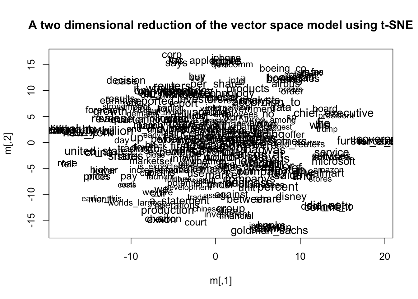
#split_news <- list()
#max_length <- 0


#for(i in 1:length(text_tidy_df$document)){
#  split_news[[i]] <- strsplit(text_tidy_df$document[i], split = ' ')
#  if(length(split_news[[i]][[1]]) > max_length){max_length <- length(split_news[[i]][[1]])}
#}


#vec_array <- array(NA, dim = c(length(text_tidy_df$document), vec_length, max_length))

#for(j in 1:length(text_tidy_df$document)){

#news_mat <- matrix(0, ncol = max_length - length(split_news[[1]][[1]]), nrow = vec_length)

#for(i in 1:length(split_news[[1]][[1]])){

#  news_mat <- cbind(news_mat, model[[split_news[[1]][[1]][i]]]@.Data[1,])

#}


#}