Chapter 2 Urban form as Predictors

2.1 Influencing Direction

Before discussing the impact of land use on travel, the first question is, does land use characteristics is the treatment affecting the outcome of travel behavior? Or the affecting direction is opposite? Technically, randomized experiments can identify the causal relationship between them. But in real life, it is impossible to setup some experimental areas and randomly assign people to live in these areas. Another way is to observe the dynamic of these factors to figure out the direction of influences.

Muller (2004) reviews the evolution of the U.S. urban form and describe the four eras of intrametropolitan growth (Figure ) in U.S. history: the walking-horsecar era (1800s – 1890s), the electric streetcar or transit era (1890s – 1920s), the recreational automobile era (1930s – 1950s), and the freeway era (1950s – 2010s) (Rodrigue, Comtois, and Slack 2016). Each of the four-stage urban transportation development has its dominated spatial structure, which is hard represented by other socio-economic concepts. Each era has the distinctive travel mode, range of distance, and land-use patterns. People can see that the innovation of transportation technology is a determining constraint to other factors and a main driving force to launch the next era.

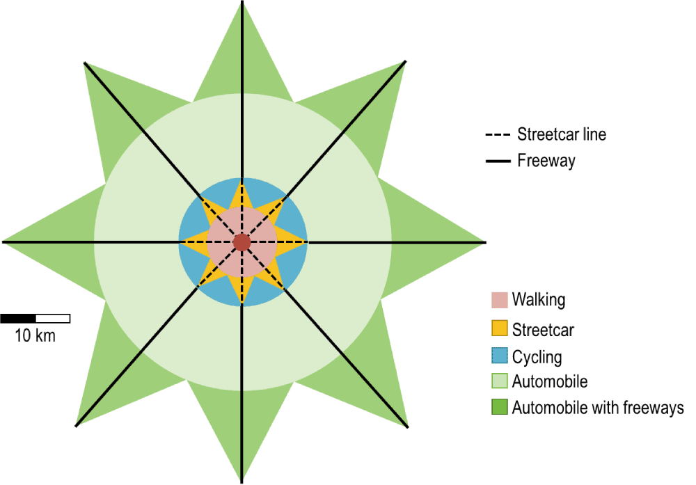
Figure 2.1: One Hour Commuting According to Different Urban Transportation Modes. Source: P.Hugill (1995), World Trade since 1431, p. 213.

New transportation tools shifted people’s travel modes, extended travel distance, and reshaped the urban form. In causal inference, the new tools is called confounder or common cause who affect both treatment and outcome. But what is the relationship between travel and land use? A simple way is to observe the sequence fo events to happen. In each transition period, the new tools and new modes began ahead of the new urban development. Even today multiple travel modes exist in old town but suburban seldom has old mode like streetcar. Thus, land use is more like a outcome rather than treatment.

However, the urban form remains relatively more stable than individual’s travel behavior in each era. A family may be used to driving in Texas and turn to use the subway when they move to New York and vice versa. Given a period, VMT could be affected by density and other factors. It doesn’t make sense that VMT will change the density in the short term. Therefore, land use can be treated as indepedent variables in the context of the current stage of urban development. The relationship of land use with respect to travel can hold for a period of time.

Over the long term, the relationships among travel, land use, and other physical, socioeconomic, demographic factors were interactive and iterative. D. M. Levinson and Krizek (2018) emphasize transportation is a necessary but not a sufficient factor for any development. The change of eras is a comprehensive outcome of socioeconomic and technological development. Which factor caused which effect does not have a simple answer. A conservative view is that land use and travel behavior are determined simultaneously by the transportation costs (Pickrell 1999).

Although randomized experiments about travel and land use are impossible, once the simultaneous relationship holds, the regression model still can explore the associations between travel and land use.

2.2 Influencing Factors

A large mount of studies try to identify the influencing factors and evaluate the effect size. Previous research demonstrated that there is not a single factor determining travel behavior. When choosing continues response, like VMT, the basic regression model is:

\[\begin{aligned} \mathbf{Y}=\mathbf{X}\boldsymbol{\beta}+\boldsymbol{\varepsilon} \end{aligned}\]

where \(\mathbf{Y}\) are the variable of VMT. \(\mathbf{X}\) are all relevant covariates with corresponding coefficients \(\boldsymbol{\beta}\). \(\boldsymbol{\varepsilon}\) are a random error terms with expected value of \(0\) and variance \(\sigma^2\).

When the response is categorical variable, such as binary data of driving versus not, polytomous data of mode choice, or count data of trip frequency, the proper model is:

\[\begin{aligned} E[\mathbf{Y}|\mathbf{X}]=\mu=g^{-1}(\mathbf{X}\boldsymbol{\beta}) \end{aligned}\]

Where \(E[\mathbf{Y}|\mathbf{X}]\) is the expected value of individual/household-level travel variable \(\mathbf{Y}\) conditional on \(\mathbf{X}\); \(\mathbf{X}\boldsymbol{\beta}\) is a linear combination (Ditto.); \(g(\cdot)\) is a link function.

For the complexity of travel behavior, many other objective or subjective factors could change people’s travel decisions. They include but are not limited to physical, socio-demographic, individual, and policy determinants. It seems impossible to make an exhaustive list.

A dichotomy of individual versus environmental factors is a most common framework. All relevant factors involving personal or household characteristics is treated as internal factors. While the built-environment and other environmental factors have external influences. Disaggregate analysis usually chooses this structure because the models can distinguish the different sources of variation from individual and environmental factors. Take for example VMT models, the model is as follow.

\[\begin{aligned} \mathbf{Y}=\mathbf{X}_\mathrm{I}\boldsymbol{\beta}_\mathrm{I}+\mathbf{X}_\mathrm{E}\boldsymbol{\beta}_\mathrm{E}+\boldsymbol{\varepsilon} \end{aligned}\]

where \(\mathbf{X}_\mathrm{I}\) are travelers’ internal characteristics; \(\mathbf{X}_\mathrm{E}\) are built environment and other environment covariates.

Previous research have identified many internal factors such as employment status, income level, lifecycle stage, habits, and preferences, having strong impact on travel. Therefore, a sufficient model should contain these influencing factors. One purpose is to increase the explanatory power. Another purpose is to control self-selection and other independent variables.

Although the internal factors, psychological, socio-demographic, and economic characteristics contribute the primary variation in these models, urban studies’ attentions are on built-environment factors such as urban density, design, and transit services. Because these factors can be intervened by policies and planning. This part of discussion will be placed in the next section separately.

At the macro scale, the concepts of ‘land use’ and ‘urban form’ are often exchangeable, The same thing is about ‘land use’ and ‘built environment’ at the meso and micro scales.

“Attributes of the built environment influence travel by making travel to opportunities more or less convenient and attractive” (Domencich and McFadden 1975; D. M. Levinson, Marshall, and Axhausen 2017; Litman 2017).

The research purpose of travel behavior is not only to describe travel itself, but also to find some tools to affect people’s behavior. Land Use is the primary focus of attention because policy or planning might be able to intervene current and future land use, further achieve the goal of behavior change.

2.2.1 Density

Density is the first built-environment factor added to the model. Early research of automobile trips and urban density can go back sixty years (Mitchell and Rapkin 1954). H. S. Levinson and Wynn (1963) suggest that the people who lived in high-density neighborhoods make fewer automobile trips. This argument stimulated an enormous volume of work. Although later studies construct more complex models, density factor stays in most of built environment-travel model even today.

The most influential aggregate studies start from Newman and Kenworthy. They published a series of studies to show a strong negative correlation between per capita fuel use and gross population density (GPD).⁴ Their sample covers from thirty-two to fifty-eight global cities (P. G. Newman and Kenworthy 1989a; P. Newman and Kenworthy 2015) and produced very convincing results. Their research points out the relationship rather than estimating the effect size. In this way, the denser cities have less fuel consumption, which implies less automobile dependence. This is a succinct argument and is widely accepted by planners and policy makers.

The criticisms include their ideological grounds, dataset, and model specification⁵. A criticism is that, for aggregated data, the population variable on both sides of the equation artificially creates a hyperbolic function (Equation (2.1)). In many disaggregated studies, the effects of density are not significant and have a small magnitude.

\[\begin{equation} \begin{split} & \text{VMT}_{average} =\beta\cdot \text{Density} +\cdots\\ \implies & \frac{\text{VMT}_{total}}{\text{Population}} = \beta\cdot \frac{\text{Population}}{\text{Area}} +\cdots\\ \implies & \text{VMT}_{total} = \beta\cdot \frac{(\text{Population})^2}{\text{Area}} +\cdots \end{split} \tag{2.1} \end{equation}\]

Another criticism argues that the global comparisons are not valid, such as comparing Hong Kong and Houston. Reid Ewing et al. (2018) created a subset with only US Metropolitan areas from Jeffrey R. Kenworthy and Laube (1999) ‘s original data set. They fit the same model but get a much lower \(R^2\) (0.096) than Kenworthy and Laube’s (0.72). A similar work by Fanis (2019) shows the low \(R^2\) for US cities (0.1838) and European cities (0.2804) when deconstructing Newman and Kenworthy’s data by continent. Actually, any research question has its corresponding sampling design. Choosing a cutoff from the whole data often gets a different result. These criticisms are unfair for Kenworthy and Laube’s work. But it is true that the US cities have higher VMT and lower density than other countries’ cities. Recent evidence over a 20-year period from other cities and counties show that the status quo of the U.S. only represents a small window of the global trend(Jeffrey R. Kenworthy 2017).

Density variable have some advantages. Density is calculated by population size and area size from census data, which are widely available over the country. In contrast, some individual variables are not as measurable and accurate as density. Some studies found density might be an intermediate variable or proxy to other land use variables such as land use mix, street network, and transit services (Reid Ewing and Cervero 2010; Handy 2005). The divisions of the statistical units in the U.S. are from an uniform criteria at multiple scales. Thus, density values is more objective, and comparable comparing other measurements.

Density is an informative factor. Except for the mean and variance, The moments function for Urban density such as skewness, kurtosis, or rank, all can be the predictor candidates. Scolar also explore more delicate measurements of density such as Propotional Weighted Density to replace overall density. “population-weighted density is equal to conventional density plus the variance of density across the subareas used for its calculation divided by the conventional density” (Ottensmann 2018). Some studies use a geographically weighted regression (GWR)⁶ procedure to identify significant employment density peaks.

Urban density can be represented by many approximate variables – built-up density, residential density, employment density, destination density, or CBD density. Here this paper focus on population density – how many people live in a square mile of land - and involves others if possible.

2.2.2 D-variables

One trenchant criticism of Newman and Kenworthy’s work is that the univariate or bivariate models may leave some critical factors out. In a recent debate (Fanis 2019), Newman clarified that “All our work shows that there are multiple causes of car dependence and multiple implications.” Since travel behavior is a multi-dimensional issue, more socio-demographic and built environment variables were added to the multivariate analysis. The work started from adding three ‘Ds’ variables, density, diversity, and design (Cervero and Kockelman 1997), extended to five ‘Ds,’ adding destination accessibility and distance to transit (Reid Ewing and Cervero 2001). It even grows to seven with the addition of demand management and demographics (TODO).

Ds’ Framework is a significance-centered mixed factor sets and becomes one of the most influential ideas among the built environment–travel literature in the past decades. Using household-level or person-level data, these studies tried to disclose more complex relationships among the candidate factors by adding more relevant variables.

The criticism from Handy (2018) says the 5Ds variables may not be independent. A meta-analysis found that spatial multicollinearity is widespread in this field (Gim 2013). Although previous studies usually check multicollinearity issues, these variables still correlate with each other in some ways and may have strong interaction effects.

2.2.3 Synthesized Index

To address the multicollinearity and interactions issues, Clifton (2017) suggest to convert the various environmental characteristics to built environment indices. Some research try to use ‘compactness indices’ to replace the single density measurement.⁷ The primary method is principal components analysis (PCA) or principal components regression (PCR), which synthesizes many variables to four dimensions: development density, land use mix, activity centering, and street connectivity. The advantage of this method is to increase the elasticity value significantly. A recent study shows that the elasticity of VMT with respect to a county compactness index is -0.78. The disadvantage of this method is that the internal mechanisms of the indices are still not clear. Another disadvantage is that the various indices are not comparable. For example, the Urban Liveability Index (ULI) by Higgs et al. (2019) includes many indicators supporting health and wellbeing. The association between ULI and travel mode choice is a specific result unless it is widely applied on other studies and cities.

A smart application of synthesize method (common factor analysis) is to control the physiological effects in models. Hong, Shen, and Zhang (2014) convert eight attitudinal questions in the 2006 Household Activity Survey to three factors: Ease, Convenience, and Pro-transit. They fit the model using two geographic scales: 1-km buffer and traffic analysis zone (TAZ). After contolling the attitudinal effects, the nonresidential density and distance from CBD have significant effects on VMT at the TAZ level.

2.2.4 Meta-Aanalysis

To get a general, comparable outcome, Reid Ewing and Cervero (2010) collect more than 200 related studies and try to summarize the elasticity values using meta-analysis. Elasticity measures the percentage change in response with respect to a 1 percent increase in a predictor. Thus, it is a dimensionless parameter. After screening, sixty-two studies were selected. But divided by modes (VMT, walking, and transit use), only nine studies were used to calculate the weighted-average elasticities of VMT with respect to population density. Of nine papers, six gave zero or insignificant elasticity, while three showed significant negative values (two are -0.04 and one is -0.12). The weighted-average elasticity of job density (sample size = 9) was zero. The largest elasticity of VMT belonged to Destination accessibility, -0.20 with respect to Job accessibility by auto (sample size = 5) and -0.22 with respect to Distance to downtown (sample size = 3). Due to the small sample size, the confidence intervals were not available. The authors call for more relevant studies to refine the results.

Stevens (2017a) also try to explain the different outcomes using a meta-regression method. Based on the results from 37 studies, they found the magnitude of effects is small and suggest that compacting development has a tiny influence on driving. His work triggers a new round of discussion (Handy 2017; Knaap, Avin, and Fang 2017; Nelson 2017; Manville 2017; Clifton 2017)

In Reid Ewing and Cervero (2017) ‘s reply, they agreed with the values of elasticity but emphasize that Stevens’ results (-0.15 ~ -0.22) are not small actually. In a forthcoming study by Ewing and Cervero, an update elasticity of VMT per capita with respect to density is -0.15 (Reid Ewing et al. 2018). In Stevens (2017b) ’s response to commentaries , he clarified the research goals and important questions.

After the two milestones for meta-analysis of built environment and travel behavior, a recent update re-examines the post-2010 empirical literature and summarized the most common factors (Aston et al. 2021). They are Density, Urban design, Local land use mix, mono/polycentrism and centrality, and Regional jobs-housing balance

2.2.5 Other Factors

2.2.5.1 Individual Factors

Here briefly introduces several significant influencing factors.

• Income levels

• Vehicle ownership

• Working status

• Major life events/lifecycle

Some major life events, such as transitions to higher school, labor market, marriage, parenthood, retirement, and relocation, could provide windows of opportunity for travel behavior change (Larouche et al. 2020). The results of a scoping review show that relocation prompts people to reflect on their travel behaviors. Entry into the labor market often increases driving while retirement may have more walking or cycling for fewer time constraints. The effects of school transition may have different directions due to the environmental differences. Marriage is not significant because couples may live together before marriage. In a similar way, parents may have more car use several years after childbirth for the purposes of childcare, school, recreation, etc.

• Psychological factors

• Attitude

• Habit

2.2.5.2 Environmental Factors

• Natural Environment

Physical Environment and other factors

• Infrastructure supplement

Infrastructure supplement is also a set of strong explanatory variables. It has been proven that road capacity and parking space

• policy interventions

(e.g., restrictions on car use) Travel Demand Management (TDM): The levels of land use policy tools. “largely remain under a local government’s authority,” “This imbalanced institutional setting and fragmented government system”

Urban Development Policies (UBG,TOD, Zoning)

There are many complex unknown interaction effects between individual and environmental variables. Some research found that the habit discontinuity hypothesis, major life events may provide windows of opportunity during which individuals may reconsider their travel behaviors and be more sensitive to behavior change interventions (Verplanken et al. 2008). Similarly, ‘changes in built environment attributes may be particularly salient for behaviour change following relocation.’

2.3 Spatial Scales

Due to the various data sources or research interests, built environment-travel studies divide into two groups. One group uses aggregated travel and built-environment variables at the city, county, or metropolitan level. At the same time, the other group uses trip data at the individual or household level.

Research also find that the models at different scales would give different result. This phenomenon is called Modifiable areal unit problem (MAUP). Previous studies found that the density variables evaluated at different spatial scales have different impact on travel (Boarnet and Crane 2001; Buchanan et al. 2006; Sultana and Weber 2007). It is not reasonable to neglect the scale issues in built environment-travel studies.

2.3.1 Urban/Region Scale

Tradition of aggregate analysis treat a city or metropolitan as an observation. Both dependent and independent variables are aggregated at macro level. Here the land use factors only reflect the density, pattern and structure at the whole city.

Coevering and Schwanen (2006) carry on Newman and Kenworthy’s work and consider four sets of potential explanatory variables: ten of urban form, six of transport service, five of housing and development history, and thirteen of socio-economic situations. They fit some linear regression models (all the variables keep the initial magnitude without taking logarithm or other transformation) and all of their adjusted \(R^2\) are higher than 0.7. Their models also show that the cities with higher population density drive less. They found the land use characteristics of the inner area are more important than metropolitan-wide population density. Similarly, a recent city-level study (Gim 2021) fit multiple regression models based on the data from 65 global cities. The population density becomes not significant in this model. Their results show that fuel price, household size, and congestion level have strong effects on travel time. Using structural equation modeling, they also find the population density of the high-density built-up areas has a larger effect on travel than overall city density.

The aggregate models confound the individual level’s variance. Urban form factors usually show significant effect.

2.3.2 Neighborhood Scale

In disaggregate analysis, the travel records by individual or household are the basic unit of dependent variables. traveler’s socio-demographic characteristics also keep this resolution such as income and vehicle ownership. However, built environment factors technically have a minimum geographic unit as the measure scope. Census tract and block group are the most common unit in disaggregate analysis.

Scholars who choose disaggregate analysis believe that the internal difference of urban characteristics be neglected at region level. They are interested in the impact of meso-level built-environment factors like the population and employment distribution of intra-urban.

Using disaggregate data can disclose the neighborhood-level differences and eliminate aggregation bias. Using logarithms of VMTs per vehicle from National Personal Travel Survey (NPTS) data with 114 urban areas, Bento et al. (2005) fit the linear model with 19 variables. They found that, instead of population density, population centrality has a significant effect on VMT. The elasticity of annual VMT with respect to population centrality is 1.5.⁸

The results of travel models at different scales are often inconsistent. Using the same data source, Reid Ewing et al. (2018) found that the elasticities of VMT with respect to population density is -0.164 in the aggregate models, which is a much higher value than disaggregate studies (-0.04 in the meta-analysis of Reid Ewing and Cervero (2010)). They suspect that this phenomenon is aggregation bias or ecological fallacy. They further explain that the two scales represent two different questions: The metropolitan-level density, which strongly affects the VMT, is not equivalent to the neighborhood density, which has much weaker effects on VMT.

2.3.3 Multi-scale Studies

Schwanen, Dieleman, and Dijst (2004) explains that many urban form dimensions are tied to specific geographical scales. Recently, more studies import the spatial scales as an explanatory variable. In a report of travel and polycentic development, Reid Ewing et al. (2020) identify 589 centers in 28 U.S. regions. Then a categorical variable, ‘within/outside a center’ is added into the model. The results show that the household living within a center have more walk trips and fewer VMT than who living outside a center.

S. Lee and Lee (2020) also conduct a study involving factors at three level: household, census tract, and urbanized area. They find that density and centrality affect VMT at urban level as well as the meso-scale jobs-housing mix. After controlling for factors, the effect of local factors the urban-level spatial structure moderates the effects size of local built environment on travel.

2.3.4 Modifiable areal unit problem (MAUP)

Early in 1930, scholars noticed that, when a set of smaller areal units was aggregated into larger areal units, the variance structure will be changed and the estimated coefficients will be larger (Gehlke and Biehl 1934). This inconsistency/sensitivity of analysis results is called modifiable areal unit problem (MAUP) and ecological fallacy (Openshaw 1984).

In aggregated analysis, two kinds of MAUP often happen simultaneously (Wong 2004). The first one called ‘scale effect’ means that the correlation among variables depends on the size of areal units. Larger units usually lead to larger estimations. The second one, zone effect describe the various results of correlation by choosing different areal shape or subset at the same scale.

Fotheringham and Wong (1991) found that multivariate analysis is unreliable when using the data from areal units. Both value and direction of estimated coefficients may change for different spatial configurations (G. Lee, Cho, and Kim 2016; Xu, Huang, and Dong 2018).

Meanwhile, some aggregate studies shows that, using the simple averages of individual data, the estimations of coefficients in linear model are unbiased (Prais and Aitchison 1954). A condition is that the regression model must fix the omission error using proper specification (Amrhein 1995; Ye and Rogerson 2021). The check of unit consistency may help to examine the biases by MAUP on the estimations.

2.4 Summary

The factors measured at a specific scale could only explain the variation generated at or above that level. Even some factors such as density has cross scales. Their distributions in different units and scales are not identical. It is reasonable for them to have various meanings and influences on travel. A systematic comparison should be conducted among multi-scale studies. The inconsistent might not be about correct or wrong. As Reid Ewing et al. (2018) commented, the aggregate and disaggregate studies are asking the apples and oranges questions.

References

Amrhein, C G. 1995. “Searching for the Elusive Aggregation Effect: Evidence from Statistical Simulations.” Environment and Planning A: Economy and Space 27 (1): 105–19. https://doi.org/10.1068/a270105.

Aston, Laura, Graham Currie, Alexa Delbosc, Md Kamruzzaman, and David Teller. 2021. “Exploring Built Environment Impacts on Transit Use an Updated Meta-Analysis.” Transport Reviews 41 (1): 73–96. https://doi.org/10.1080/01441647.2020.1806941.

Bento, Antonio M., Maureen L. Cropper, Ahmed Mushfiq Mobarak, and Katja Vinha. 2005. “The Effects of Urban Spatial Structure on Travel Demand in the United States.” The Review of Economics and Statistics 87 (3): 466–78. https://doi.org/10.1162/0034653054638292.

Boarnet, Marlon, and Randall Crane. 2001. “The Influence of Land Use on Travel Behavior: Specification and Estimation Strategies.” Transportation Research Part A: Policy and Practice 35 (9): 823–45. https://doi.org/10.1016/S0965-8564(00)00019-7.

Buchanan, Nick, Ross Barnett, Simon Kingham, and Doug Johnston. 2006. “The Effect of Urban Growth on Commuting Patterns in Christchurch, New Zealand.” Journal of Transport Geography 14 (5): 342–54. https://doi.org/10.1016/j.jtrangeo.2005.10.008.

Cervero, Robert, and Kara Kockelman. 1997. “Travel Demand and the 3Ds: Density, Diversity, and Design.” Transportation Research Part D: Transport and Environment 2 (3): 199–219. https://doi.org/10.1016/S1361-9209(97)00009-6.

Clifton, Kelly J. 2017. “Getting From Here to There: Comment on “Does Compact Development Make People Drive Less?”.” Journal of the American Planning Association 83 (2): 148–51. https://doi.org/10.1080/01944363.2017.1290494.

Coevering, Paul van de, and Tim Schwanen. 2006. “Re-Evaluating the Impact of Urban Form on Travel Patternsin Europe and North-America.” Transport Policy 13 (3): 229–39. https://doi.org/10.1016/j.tranpol.2005.10.001.

Domencich, T. A., and D. McFadden. 1975. “URBAN TRAVEL DEMAND - A BEHAVIORAL ANALYSIS.” http://trid.trb.org/view/48594.

Dujardin, S., F. Pirart, F. Brévers, A. -F. Marique, and J. Teller. 2012. “Home-to-Work Commuting, Urban Form and Potential Energy Savings: A Local Scale Approach to Regional Statistics.” Transportation Research Part A: Policy and Practice 46 (7): 1054–65. https://doi.org/10.1016/j.tra.2012.04.010.

Ewing, Reid, and Robert Cervero. 2001. “Travel and the Built Environment: A Synthesis.” Transportation Research Record: Journal of the Transportation Research Board 1780 (January): 87–114. https://doi.org/10.3141/1780-10.

———. 2010. “Travel and the Built Environment.” Journal of the American Planning Association 76 (3): 265–94. https://doi.org/10.1080/01944361003766766.

———. 2017. ““Does Compact Development Make People Drive Less?” The Answer Is Yes.” Journal of the American Planning Association 83 (1): 19–25. https://doi.org/10.1080/01944363.2016.1245112.

Ewing, Reid, Shima Hamidi, and James B Grace. 2016. “Urban Sprawl as a Risk Factor in Motor Vehicle Crashes.” Urban Studies 53 (2): 247–66. https://doi.org/10.1177/0042098014562331.

Ewing, Reid, Shima Hamidi, Guang Tian, David Proffitt, Stefania Tonin, and Laura Fregolent. 2018. “Testing Newman and Kenworthy’s Theory of Density and Automobile Dependence.” Journal of Planning Education and Research 38 (2): 167–82. https://doi.org/10.1177/0739456X16688767.

Ewing, Reid, Gail Meakins, Shima Hamidi, and Arthur C. Nelson. 2014. “Relationship Between Urban Sprawl and Physical Activity, Obesity, and Morbidity Update and Refinement.” Health & Place 26 (March): 118–26. https://doi.org/10.1016/j.healthplace.2013.12.008.

Ewing, Reid, Keunhyun Park, Sadegh Sabouri, Torrey Lyons, Keuntae Kim, Dong-ah Choi, Katherine Daly, and Roya Ghasrodashti. 2020. “Reducing Vehicle Miles Traveled, Encouraging Walk Trips, and Facilitating Efficient Trip Chains Through Polycentric Development.” TREC Final Reports, October. https://doi.org/10.15760/trec.255.

Fanis, Grammenos. 2019. “Three Studies That Show Density Doesn’t Determine Car Travel.” Planetizen - Urban Planning News, Jobs, and Education. https://www.planetizen.com/features/106433-three-studies-show-density-doesnt-determine-car-travel.

Fotheringham, A S, and D W S Wong. 1991. “The Modifiable Areal Unit Problem in Multivariate Statistical Analysis.” Environment and Planning A: Economy and Space 23 (7): 1025–44. https://doi.org/10.1068/a231025.

Gehlke, C. E., and Katherine Biehl. 1934. “Certain Effects of Grouping Upon the Size of the Correlation Coefficient in Census Tract Material.” Journal of the American Statistical Association 29 (185A): 169–70. https://doi.org/10.1080/01621459.1934.10506247.

“Geographically Weighted Regression - an Overview ScienceDirect Topics.” n.d. Accessed August 22, 2021. https://www-sciencedirect-com.proxy.lib.pdx.edu/topics/earth-and-planetary-sciences/geographically-weighted-regression.

Gim, Tae-Hyoung Tommy. 2013. “The Relationships Between Land Use Measures and Travel Behavior: A Meta-Analytic Approach.” Transportation Planning and Technology 36 (5): 413–34. https://doi.org/10.1080/03081060.2013.818272.

———. 2021. “Analyzing the City-Level Effects of Land Use on Travel Time and Co2 Emissions: A Global Mediation Study of Travel Time.” International Journal of Sustainable Transportation 0 (0): 1–18. https://doi.org/10.1080/15568318.2021.1901163.

Gordon, Peter, and Harry W. Richardson. 1989. “Gasoline Consumption And Cities: A Reply.” American Planning Association. Journal of the American Planning Association 55 (3): 342. http://search.proquest.com/docview/229599978/abstract/FBB96AB65F044006PQ/1.

Hamidi, Shima, and Reid Ewing. 2014. “A Longitudinal Study of Changes in Urban Sprawl Between 2000 and 2010 in the United States.” Landscape and Urban Planning 128 (August): 72–82. https://doi.org/10.1016/j.landurbplan.2014.04.021.

Hamidi, Shima, Reid Ewing, Ilana Preuss, and Alex Dodds. 2015. “Measuring Sprawl and Its Impacts: An Update.” Journal of Planning Education and Research 35 (1): 35–50. https://doi.org/10.1177/0739456X14565247.

Handy, Susan. 2005. “Critical Assessment of the Literature on the Relationships Among Transportation, Land Use, and Physical Activity,” 102.

———. 2017. “Thoughts on the Meaning of Mark Stevens’s Meta-Analysis.” Journal of the American Planning Association 83 (1): 26–28. https://doi.org/10.1080/01944363.2016.1246379.

———. 2018. “Enough with the “D’s” Already Let’s Get Back to “A”.” Transfers Magazine, no. 1 (May). http://trid.trb.org/view/1709460.

Higgs, Carl, Hannah Badland, Koen Simons, Luke D. Knibbs, and Billie Giles-Corti. 2019. “The Urban Liveability Index: Developing a Policy-Relevant Urban Liveability Composite Measure and Evaluating Associations with Transport Mode Choice.” International Journal of Health Geographics 18 (1). https://doi.org/10.1186/s12942-019-0178-8.

Hong, Jinhyun, Qing Shen, and Lei Zhang. 2014. “How Do Built-Environment Factors Affect Travel Behavior? A Spatial Analysis at Different Geographic Scales.” Transportation 41 (3): 419–40. https://doi.org/10.1007/s11116-013-9462-9.

Kenworthy, J. R., F. B. Laube, P. Newman, P. Barter, T. Raad, C. Poboon, and B. Guia Jr. 1999. AN INTERNATIONAL SOURCEBOOK OF AUTOMOBILE DEPENDENCE IN CITIES 1960-1990. http://trid.trb.org/view/648499.

Kenworthy, Jeffrey R. 2017. “Is Automobile Dependence in Emerging Cities an Irresistible Force? Perspectives from São Paulo, Taipei, Prague, Mumbai, Shanghai, Beijing, and Guangzhou.” Sustainability 9 (11): 1953. https://doi.org/10.3390/su9111953.

Kenworthy, Jeffrey R, and Felix B Laube. 1999. “Patterns of Automobile Dependence in Cities: An International Overview of Key Physical and Economic Dimensions with Some Implications for Urban Policy.” Transportation Research Part A: Policy and Practice 33 (7): 691–723. https://doi.org/10.1016/S0965-8564(99)00006-3.

Knaap, Gerrit-Jan, Uri Avin, and Li Fang. 2017. “Driving and Compact Growth: A Careful Look in the Rearview Mirror.” Journal of the American Planning Association 83 (1): 32–35. https://doi.org/10.1080/01944363.2017.1251276.

Larouche, Richard, this link will open in a new window Link to external site, Ulises Charles Rodriguez, Ransimala Nayakarathna, and David R. Scott. 2020. “Effect of Major Life Events on Travel Behaviours: A Scoping Review.” Sustainability 12 (24): 10392. https://doi.org/http://dx.doi.org.proxy.lib.pdx.edu/10.3390/su122410392.

Lee, Gunhak, Daeheon Cho, and Kamyoung Kim. 2016. “The Modifiable Areal Unit Problem in Hedonic House-Price Models.” Urban Geography 37 (2): 223–45. https://doi.org/10.1080/02723638.2015.1057397.

Lee, Sungwon, and Bumsoo Lee. 2020. “Comparing the Impacts of Local Land Use and Urban Spatial Structure on Household VMT and GHG Emissions.” Journal of Transport Geography 84 (April): 102694. https://doi.org/10.1016/j.jtrangeo.2020.102694.

Levinson, David M., and Kevin J. Krizek. 2018. Metropolitan Transport and Land Use: Planning for Place and Plexus. 2nd ed. Second edition. New York : Routledge, 2018.: Routledge. https://doi.org/10.4324/9781315684482.

Levinson, David M., Wesley Marshall, and Kay Axhausen. 2017. Elements of Access: Transport Planning for Engineers, Transport Engineering for Planners. Network Design Lab. https://ses.library.usyd.edu.au/handle/2123/21628.

Levinson, Herbert S., and F. Houston Wynn. 1963. “EFFECTS OF DENSITY ON URBAN TRANSPORTATION REQUIREMENTS.” Highway Research Record, no. 2. http://trid.trb.org/view/133884.

Litman, Todd. 2017. “How Land Use Factors Affect Travel Behavior,” 91.

Manville, Michael. 2017. “Travel and the Built Environment: Time for Change.” Journal of the American Planning Association 83 (1): 29–32. https://doi.org/10.1080/01944363.2016.1249508.

Mitchell, Robert B., and Chester Rapkin. 1954. Urban Traffic. Columbia University Press. http://www.degruyter.com/document/doi/10.7312/mitc94522/html.

Muller, Peter O. 2004. Transportation and Urban Form - Stages in the Spatial Evolution of the American Metropolis. http://trid.trb.org/view/756060.

Nelson, Arthur C. 2017. “Compact Development Reduces VMT: Evidence and Application for PlannersComment on “Does Compact Development Make People Drive Less?”.” Journal of the American Planning Association 83 (1): 36–41. https://doi.org/10.1080/01944363.2016.1246378.

Newman, P. G., and J. R. Kenworthy. 1989a. CITIES AND AUTOMOBILE DEPENDENCE: AN INTERNATIONAL SOURCEBOOK. http://trid.trb.org/view/351194.

Newman, P. G., and Jeffrey R. Kenworthy. 1989b. “Gasoline Consumption and Cities.” Journal of the American Planning Association 55 (1): 24–37. https://doi.org/10.1080/01944368908975398.

Newman, Peter. 2014. “Density, the Sustainability Multiplier: Some Myths and Truths with Application to Perth, Australia.” https://pubag.nal.usda.gov/catalog/6516732.

Newman, Peter, and Jeff Kenworthy. 2011a. “‘Peak Car Use’: Understanding the Demise of Automobile Dependence.” World Transport Policy & Practice 17 (2). http://trid.trb.org/view/1106687.

———. 2011b. “The Density Multiplier: A Response to Mees.” World Transport Policy & Practice 17 (3). http://trid.trb.org/view/1127388.

Newman, Peter, and Jeffrey Kenworthy. 2015. “The End of Automobile Dependence:” In The End of Automobile Dependence: How Cities Are Moving Beyond Car-Based Planning, edited by Peter Newman and Jeffrey Kenworthy, 201–26. Washington, DC: Island Press/Center for Resource Economics. https://doi.org/10.5822/978-1-61091-613-4_7.

Newman, Peter, Jeffrey Kenworthy, Peter Newman, and Jeffrey Kenworthy. 2006. “Urban Design to Reduce Automobile Dependence.” Opolis, 35–52.

Openshaw, S. 1984. “Ecological Fallacies and the Analysis of Areal Census Data.” Environment and Planning A: Economy and Space 16 (1): 17–31. https://doi.org/10.1068/a160017.

Ottensmann, John R. 2018. “On Population-Weighted Density.” {SSRN} {Scholarly} {Paper} ID 3119965. Rochester, NY: Social Science Research Network. https://doi.org/10.2139/ssrn.3119965.

Perumal, Andrew, and David Timmons. 2017. “Contextual Density and US Automotive Co2 Emissions Across the RuralUrban Continuum.” International Regional Science Review 40 (6): 590–615. https://doi.org/10.1177/0160017615614897.

Pickrell, D. 1999. TRANSPORTATION AND LAND USE. http://trid.trb.org/view/500082.

Prais, S. J., and J. Aitchison. 1954. “The Grouping of Observations in Regression Analysis.” Revue de l’Institut International de Statistique / Review of the International Statistical Institute 22 (1/3): 1–22. https://doi.org/10.2307/1401916.

Rodrigue, Jean-Paul, Claude Comtois, and Brian Slack. 2016. The Geography of Transport Systems. 4th ed. London: Routledge. https://doi.org/10.4324/9781315618159.

Schwanen, Tim, Frans M. Dieleman, and Martin Dijst. 2004. “The Impact of Metropolitan Structure on Commute Behavior in the Netherlands: A Multilevel Approach.” Growth and Change 35 (3): 304–33. https://doi.org/10.1111/j.1468-2257.2004.00251.x.

Stevens, Mark R. 2017a. “Does Compact Development Make People Drive Less?” Journal of the American Planning Association 83 (1): 7–18. https://doi.org/10.1080/01944363.2016.1240044.

———. 2017b. “Response to Commentaries on “Does Compact Development Make People Drive Less?”.” Journal of the American Planning Association 83 (2): 151–58. https://doi.org/10.1080/01944363.2017.1287588.

Sultana, Selima, and Joe Weber. 2007. “Journey-to-Work Patterns in the Age of Sprawl: Evidence from Two Midsize Southern Metropolitan Areas.” The Professional Geographer 59 (2): 193–208. https://doi.org/10.1111/j.1467-9272.2007.00607.x.

Verplanken, Bas, Ian Walker, Adrian Davis, and Michaela Jurasek. 2008. “Context Change and Travel Mode Choice: Combining the Habit Discontinuity and Self-Activation Hypotheses.” Journal of Environmental Psychology 28 (2): 121–27. https://doi.org/10.1016/j.jenvp.2007.10.005.

Wong, David W. S. 2004. “The Modifiable Areal Unit Problem (MAUP).” In WorldMinds: Geographical Perspectives on 100 Problems: Commemorating the 100th Anniversary of the Association of American Geographers 19042004, edited by Donald G. Janelle, Barney Warf, and Kathy Hansen, 571–75. Dordrecht: Springer Netherlands. https://doi.org/10.1007/978-1-4020-2352-1_93.

Xu, Pengpeng, Helai Huang, and Ni Dong. 2018. “The Modifiable Areal Unit Problem in Traffic Safety: Basic Issue, Potential Solutions and Future Research.” Journal of Traffic and Transportation Engineering (English Edition) 5 (1): 73–82. https://doi.org/10.1016/j.jtte.2015.09.010.

Ye, Xiang, and Peter Rogerson. 2021. “The Impacts of the Modifiable Areal Unit Problem (MAUP) on Omission Error.” Geographical Analysis n/a (n/a). https://doi.org/10.1111/gean.12269.

---

4. P. G. Newman and Kenworthy (1989a);P. G. Newman and Kenworthy (1989b);J. R. Kenworthy et al. (1999);P. Newman et al. (2006);P. Newman and Kenworthy (2011a);P. Newman and Kenworthy (2011b);P. Newman (2014);P. Newman and Kenworthy (2015);Jeffrey R. Kenworthy (2017)↩︎

5. Gordon and Richardson (1989);Dujardin et al. (2012);Perumal and Timmons (2017)↩︎

6. “Geographically Weighted Regression - an Overview ScienceDirect Topics” (n.d.)↩︎

7. Reid Ewing, Meakins, et al. (2014);Hamidi and Ewing (2014);Hamidi et al. (2015);Reid Ewing, Hamidi, and Grace (2016)↩︎

8. “population centrality measure is computed by averaging the difference between the cumulative population in annulus n (expressed as a percentage of total population) and the cumulative distance-weighted population in annulus n (expressed as a percentage of total distance-weighted population).”↩︎