Chapter 2 Introduction to Inference

2.1 Motivation
This topic can often feel unintuitive, and a lot of the uneasiness can stem from a base misunderstanding of the fundamental jargon that we build our theory on. That’s why it’s so vital to really understand the introductory concepts so that down the road, you won’t stumble on the terminology and methodology we employ. This might be the first time you have to think like a true statistician. It takes some practice, but you will get there.
2.2 Basic Terminology
Up to this point, your only statistical experience may be in probability; an excellent subject, to be sure, but one that operates in a bit of a vacuum. You’ll find that Inference provides a bridge that spans from the classroom to real-world data.
In probability, we are given distributions and parameters, and asked to find out the probability of something occurring. Consider a standard probability problem:
Three students take \(i.i.d. \; Expo(\frac{1}{10})\) minutes to finish their homework. How long on average does it take for all three students to complete their homework?
You would solve this using the memoryless property and the minimum of exponentials, but the point remains that you are given the distribution - Exponential - and given the parameter: \(\lambda = \frac{1}{10}\) minutes - and then have to calculate something based off of this info (the average time for all three to finish).
With inference, you might have the opposite problem; you might observe data for a lot of students finishing their homework (maybe you have 4 students do their homework and they take 11, 15, 9, 7 minutes each) and then estimate what the distribution is or the parameter of the distribution for the finishing times.
Believe it or not, you engage in inferential thinking all the time. Ever wonder about what the average is for anything? For example, you’ve probably been curious right after taking an exam what the average grade was. How do you approach estimating the average grade? Simple: you go around asking people how they did, collecting their reactions as data, and take that average. There are definitely issues with this method, right? For instance, people can tell you how they think they did, but they don’t know exact scores yet. Some people might be wrong. Some people might be lying! Still, it’s not a bad method to get a rough estimate of the average. Maybe you employ other methods like asking ‘average’ people how they did to get a better sense, and not asking ‘outliers’ (people you know did really well or really poorly) to avoid skewing your data. Out of a simple concept, many complexities can arise!
You’re probably starting to see what we’re talking about, and probably thinking to yourself just how often you do this. Ever wonder about average heights? Average IQs? How much variance there is in undergraduate financial aid in universities across the country? All of this is statistical inference! We’re just going to dig deep and mathematically formalize this process, finding the best approaches, solutions and tools to estimate whatever comes our way.
Now that you we an idea of what inference is all about, we’ll formalize some definitions for the holistic process that we’ll see over and over again. Make sure to get these definitions down now; there’s nothing too tricky about them when you break them down, but you will hear them so often that it’s important to be familiar with them.
Parameter - This is what it’s all about. The official definition is “a characteristic that determines the joint distribution for random variables of interest.” This definition isn’t very helpful, but just think back to probability. Remember a Normal distribution? It has a mean and a variance, right? Well, these are the parameters of the distribution; they are what govern the distribution, what sets it apart from others in the same family. For example, a \(N(0,4)\) is different from a \(N(0,6)\) because they have different variances, and variance is a parameter that governs spread. Probably the most simple parameter and the one we are most often trying to estimate is the mean.
Remember that parameters are the truth. If you’re trying to estimate the average grade on an exam like in the last example, the true average of all the scores is the parameter you’re trying to estimate. Usually, in practice, we write parameters as the Greek letter theta, or \(\theta\). You might see it written as a vector; for example, the parameters of a Normal distribution might be \(\theta = (\mu,\sigma)\). Parameters govern the model, which in turn governs the actual data. If the model for exam scores is \(N(86,4)\), then each person’s exam score is a random variable with distribution \(N(86,4)\) (this is kind of subtle but pretty important, so spend some time thinking about it. Each individual in the population, under the general assumptions that we have, will be a random variable governed by the population model. Here the population model was \(N(86,4)\). More on this later).
Parameter Space - Much like the sample space, this gives all values that a parameter can take on, and is denoted \(\Omega\). For example, if the parameter of interest is the true mean of scores on an exam (and the exam is out of 100 points) the true mean could be anywhere from 0 to 100, so the interval \((0,100)\) inclusive is the parameter space.
Statistic - The formal definition is a ‘function of random variables’; again, this is not too instructive. Think about a statistic as any ‘summary number’ for data that you’re interested in. For example, if we’re going back to looking at exam grades, the maximum exam grade is a statistic. So is the median grade. So is the average grade plus 7. Get it? They’re all just functions of the data, and they all tell us something slightly different. You’ve probably heard of “summary statistics” before; same idea, just statistics like the mean and median that do a good job of summarizing a dataset. Why are they functions of random variables? Well, recall that the data crystallizes from random variables. If the statistical model is that the true waiting time for a bus is \(Expo(\frac{1}{10})\), for example, then each waiting time is a \(Expo(\frac{1}{10})\) random variable, and the data we observe are just outcomes from these random variables.
Estimator - This is a big one. The way we think of this is a tool that estimates a parameter. For example, what would be a good estimator for the true population (overall) mean of exam scores? Well, the sample mean (of the sample exam scores you observed) seems like a good choice! Here, the sample mean is the estimator because it, well, estimates the parameter of interest. We might write it as:
\[\bar{X} = \frac{1}{n}\sum_{i = 1}^n x_i\]
Where \(\bar{X}\) is the sample mean, we have \(n\) data points, and \(x_i\) is the \(i^{th}\) data point. We’re taking a sample of \(n\) data points here. Importantly, we’re using a lowercase \(x_i\), which implies that we’ve observed the data (recall that we use capital letters like \(X\) to denote random variables, and lowercase letter like \(x\) to denote the values they crystallize to). So, this would be a sample mean from a sample that we’ve already collected.
Here, \(\bar{X}\) is an estimator for \(\mu\), or the parameter (in this case, the true mean; remember that we use Greek letters like \(\mu\) for parameters). Let’s perform an example in R to see how we might use the sample mean to estimate the true mean; we can use the example above of test scores that are distributed \(N(86, 4)\).
library(ggplot2)

# replicate
set.seed(0)
n <- 20

# generate and visualize
sample_means <- replicate(mean(rnorm(20, 86, 2)), n = 100)
ggplot() +
  geom_histogram(aes(x = sample_means)) +
  geom_vline(xintercept = 86) +
  xlab("Sample Mean") +
  ggtitle("100 Sample Means")
## `stat_bin()` using `bins = 30`. Pick better value with `binwidth`.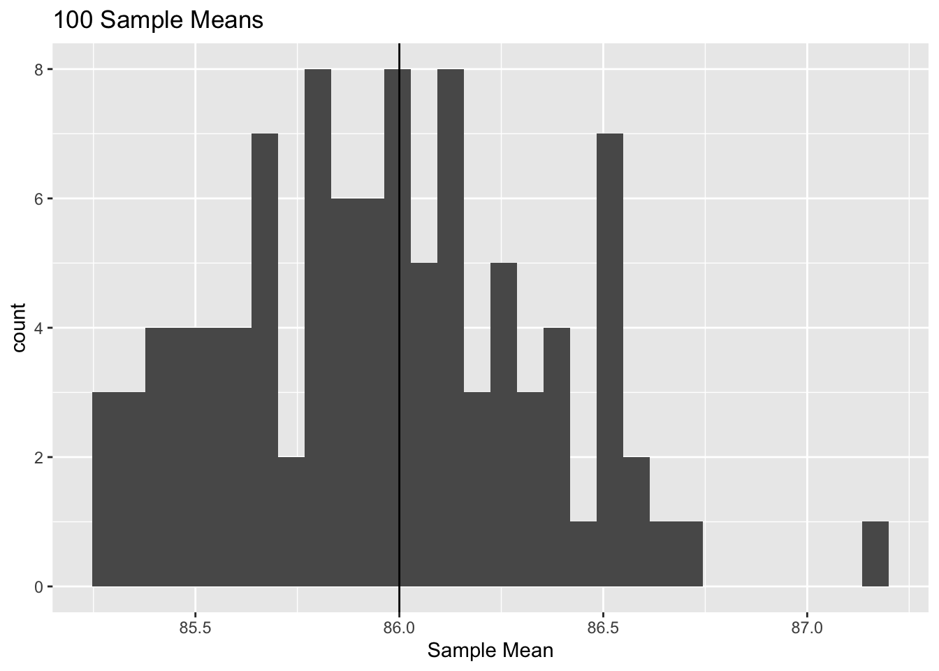
Above, we collected samples of size 20 from a population with a \(N(86, 4)\) distribution (this is the rnorm(20, 86, 2) code; we are just making 20 draws from a \(N(86, 4)\) distribution, because the ‘population model’ tells us that each person in this distribution is an i.i.d. random variable with a \(N(86, 4)\) distribution), took the mean (so that we calculated the ‘sample mean’) and replicated this whole process 100 times (that is, we collected 100 sample means from 100 different samples). We then visualize our histogram of the different sample means and see that, intuitively, they tend to cluster around the true mean of 86. Remember that, in general, we won’t know what the true mean is; it’s exactly what we are trying to estimate! This example is just provided to give you a sense of what it means to take sample means from the data intended to estimate the true parameter (the true mean).
Anyways, since estimators are just functions of the data (and, as above, we are assuming the observed data to be draws from random variables), estimators are also functions of random variables (for the sample mean, the function is to add up all of the data points and divide by the number of data points). That means that all estimators are statistics, since both are just functions of random variables! However, not all statistics are estimators.
Does this make sense? Well, an estimator is something that estimates a parameter in the model. Consider the statistic ‘median score plus 7.’ That’s a function of the data, sure (the function is take the median and add 7), but does it estimate anything worthwhile? Does it estimate a parameter that governs the model? No, it doesn’t, and so it’s not an estimator. Estimators are usually means, variances, or something similar; aimed at gauging things that govern distributions.
Estimate - Since estimators are random variables, estimates are the values they crystallize to. You can think of how we used the notation \(X\) (capital letter) in probability to denote random variables, and \(x\) (lowercase letter) to denote the value that the random variable crystallizes to; we have the same thing here. The estimate is just what we get when we plug the actual data we observe into our estimator. Therefore, the same estimator can yield different estimates for different processes, just like random variables can yield different value when you draw from them multiple times.
i.i.d. - Shorthand for “identically and independently distributed.” You likely remember this from probability: if two things are i.i.d., they have the same distribution but are independent. It’s a pretty neat property, but why are we going over it here?
We’re going to deal with joint distributions a lot in inference, so i.i.d. random variables are your friend. That’s because, as you remember, if two random variables are independent, then the joint PDF is just the product of the two marginal PDFs (similar to how if two events are independent, then the probability of their intersection - both of them occurring - is the product of the marginal probabilities). If they have the same distribution, then it’s just the PDF squared! So, if we have i.i.d. things and we need a joint distribution, we just write this big, huge product of density functions (which you will get very, very used to).
Population - You’ve probably heard of this before: a population is the entire group of individuals that we’re interested in. Populations have parameters (means, variances, etc.).
Sample- You’ve also probably heard of this: a sample is just a subset of the entire population that we collect to make estimates about the population (i.e., you take a sample of kids after an exam to guess at the population average).
Unbiased Estimators - Now that you are familiar with estimators and parameters, the idea of being ‘unbiased’ should make more sense.
An estimator is unbiased if its expectation is equal to the parameter it’s trying to estimate. This helps to remind us that estimators are random variables; we’re taking an expectation!
Let’s do a simple example with the estimator you know the best: the sample mean. We know that the sample mean is trying to estimate the true mean, \(\mu\), so let’s just use brute force and see if its expectation is equal to \(\mu\).
Recall that \(\bar{X}\), the sample mean, is:
\[\bar{X} = \frac{1}{n}\sum_{i = 1}^n X_i\]
Notice that we’re using capital \(X_i\) in the sum here instead of \(x_i\) as before. That’s because we are interested in the expectation of the random variable, the sample mean, before it crystallizes. That is, we want the expectation before we take the sample. Once we take the sample, we know the sample mean with total certainty! We don’t want one specific sample mean, though, we want what the average sample mean will be (yes, it’s very weird to think about what the average of an average will be. Remind yourself that the sample mean is a random variable that fluctuates as we take different samples of the data!). Anyways, taking the expectation yields:
\[E(\bar{X}) = E(\frac{1}{n}\sum_{i = 1}^n X_i) = \frac{1}{n}E(\sum_{i = 1}^n X_i) = \frac{1}{n}\sum_{i = 1}^n E(X_i) = \frac{1}{n} \frac{\mu}{n} = \mu\]
This employs linearity of expectation and symmetry (the expectation of every \(X_i\) should be the same, because at this point we don’t have any information that distinguishes one person from another). It also relies on the fact that the expectation of every data point, or \(E(X_i)\) is \(\mu\); this makes sense, because the true mean, the parameter, that governs the population is \(\mu\), so every individual in the sample is a random variable with mean \(\mu\). If you get confused here, take it a step back and try the process again to really hammer it down. Remember how we said that each person in the population was a random variable governed by the model? Here, the model has a mean \(\mu\), so each person is an r.v. with mean \(\mu\).
We can investigate this with our R code above; the mean of the sample means should be close to the true mean of 86, and, indeed, it is!
# replicate
set.seed(0)
n <- 20

# generate and visualize
sample_means <- replicate(mean(rnorm(20, 86, 2)), n = 100)
mean(sample_means)
## [1] 85.95938Anyways, \(\bar{X}\) is unbiased because \(E(\bar{X}) = \mu\), or, on average, the sample mean will be equal to the true mean that it is trying to estimate. This is a subtle but powerful result; it makes sense that we want our estimator to have an expectation that is the correct value. Having a biased estimator (the expectation does not equal the parameter of interest) is clearly not ideal, since on average the estimator will be wrong!
Unbiased estimators are also kind of weird because, at this moment in time, it’s hard to imagine an estimator that is not unbiased (that is, a biased estimator). Since we’ve only looked at sample means, it seems pretty obvious and easy to get an unbiased estimator - obviously the sample mean is going to, on average, be the true mean. Don’t worry; you will see biased estimators down the road!
At this point, you have all of the basic methodology to understand the base process for Inference. Let’s think of an example. Say you wanted to know the true average number of nights that a college student goes out per week; the parameter. Obviously, because of money and time constraints, you can’t find out the number of nights that every student goes out, put that in an Excel sheet, and find the average. You’ll only be able to ask a sample of the entire college population. You’ll also need an estimator, which will be a function of the data from your sample, that will estimate the parameter of interest: the true average of the number of nights out per week. The estimator you’ll probably use is the sample mean, which seems to work because it’s unbiased for the population mean (its expectation is the population mean). You’ll get data from the sample, plug the data into the function (the function is the sample mean, so add up all the values and divide by the number of values) and get your estimate for the true parameter.
Sampling Distributions - This is the distribution for a statistic (remember, a statistic is just a numerical summary of the data) given an underlying distribution with a specific parameter.
This might seem confusing at first. Let’s consider two of our favorite, and the most commonly used, estimators here: the sample mean and the sample proportion (we’ll talk about the second one soon). We’re interested in the distribution of the sample mean here. What famous distribution will that likely be? Well recall the CLT (Central Limit Theorem), which states that if we add up enough random variables, the distribution of the sum becomes Normal. So, it’s safe to say with a large enough sample, that the sample mean is Normal, because remember that each person in the population is treated as a random variable (and to take a sample mean we add them all up, before dividing by the number of people).
If the sample mean is Normal, then it has two parameters: a mean and a variance. Our job, then, is to find this mean and variance. Recall that we are finding the distribution of this estimator given the parameters of the underlying data; so here, we’ll condition on these parameters, and call them \(\mu\) and \(\sigma^2\) for the mean and variance, respectively (remember, this is the mean and variance of the population, so these are both parameters).
We already showed that the mean, or expectation, of the sample mean is \(\mu\), the population mean, since the sample mean is unbiased for that parameter. The proof is above, but that means \(E(\bar{X}) = \mu\). What about the variance? Well, let’s just use brute force to find the variance of the sample mean:
\[Var(\bar{X}) = Var(\frac{1}{n}\sum_{i = 1}^{n} X_i) = \frac{1}{n^2} Var(\sum_{i = 1}^{n} X_i) = \frac{1}{n^2}\sum_{i = 1}^{n} Var(X_i) \]
\[= \frac{1}{n^2} nVar(X_i) = \frac{1}{n}Var(X_i) = \frac{\sigma^2}{n}\]
For this proof, recall that \(Var(aX) = a^2Var(X)\). We also used symmetry, so the variance of all \(X_i\)’s are the same, and the fact that \(X_i\)’s are i.i.d. (by assumption) means that the variance of the sum is just the sum of the variances (if they weren’t independent, we’d have to deal with Covariance terms). Then, we know that \(Var(X_i) = \sigma^2\), because we’re given \(\sigma^2\) as the variance that governs the population, or, in other words, every individual in the population is a random variable with variance \(\sigma^2\). We can check that these values are close with our 4 code:
# replicate
set.seed(0)
n <- 20

# generate and visualize
sample_means <- replicate(mean(rnorm(20, 86, 2)), n = 100)
var(sample_means); 4 / n
## [1] 0.145233## [1] 0.2Anyways, we found that \(E(\bar{X}) = \mu\) and \(Var(\bar{X}) = \frac{\sigma^2}{n}\). Since we know that \(\bar{X}\) is Normal (by the CLT, since we’re adding a bunch of random variables up), and we know the parameters, we can write:
\[\bar{X} \sim N(\mu, \frac{\sigma^2}{n})\]
Where, again, \(\mu\) is the true population mean and \(\sigma^2\) is the true population variance.
You may have seen this result before in probability, but it’s neat to view through an inference lens. It’s weird to think of the sample mean as a random variable (remember that every sample is random, and the sample mean is a function of these random values, so it makes sense that it’s a random variable) and even weirder to assign it with this specific distribution!
Does the distribution make sense? Well, it’s centered around the true mean, \(\mu\), which makes sense, because we know that the sample mean is unbiased for the true population mean. How about the variance? Well, recall that \(n\) is just our sample size. Our variance, then, gets smaller as \(n\) grows. When \(n\) is very large, the variance gets close to 0, which makes sense, because as the sample gets bigger it gets closer and closer to being the true population, and thus the sample mean is more and more likely to be close to the population mean!
Let’s find the sampling distribution for another estimator: the sample proportion. Up until now, we’ve considered quantitative data: how high did someone score? How tall are they? How many points did they get? Now, let’s consider categorical data. What if instead of wanting to know the average number of nights per week that college students go out, you wanted the proportion of college students that go out on Friday nights?
Here, the parameter of interest is the population proportion, or the proportion of individuals in the entire population that satisfy some characteristic (here, going on Friday night). Say you have a sample of people and you ask if they go out on Friday. A natural estimator from this sample for the actual population would be the sample proportion, or the proportion of individuals in the sample that satisfy the characteristic.
Let’s define the sample proportion as \(\hat{p} = \frac{X}{n}\), where \(X\) is the number of individuals with the certain characteristics in the sample (here, the number of people that go out on Friday nights) and \(n\) is the size of the sample. Quick notation point: we put hats on things when we want to indicate something is the estimator. So, \(\hat{m}\) is the estimator for \(m\).
Clearly, \(\hat{p}\) is an estimator for the parameter “true population proportion.” If we want the sampling distribution of the sample proportion \(\hat{p}\), we need to condition on this true parameter (the true population proportion). Let’s say that the true population proportion is \(p\) (much like how early we used \(\mu\) as the true population mean) and that there are \(N\) people in the population, where \(N >> n\) (the population size is much greater than the sample size).
So, let’s find the distribution of \(\hat{p}\). Again, \(\hat{p}\) is just the sum of multiple random variables (each individual basically says “yes” or “no” in this study, which is a Bernoulli random variable). So, by the CLT, if \(n\) is large enough, \(\hat{p}\) follows a Normal distribution:
What’s left, then is finding the mean and variance of the estimator \(\hat{p}\). Remember that we said \(\hat{p} = \frac{X}{n}\), where \(X\) is the number of individuals with the characteristic in the sample, and \(n\) is the sample size. Let’s say that \(X = I_1 + I_2 + ... + I_n\), where \(I_i\) is the indicator that the \(i^{th}\) person in the sample has the specific characteristic. Recall that, by the Fundamental Bridge, \(E(I_i) = p\) for all \(i\). That is, the probability that each person has the specific characteristic is the probability given by the population parameter. We could also say that \(I_i \sim Bern(p)\) for all \(i\). Now, we can find the expectation and variance of \(\hat{p}\).
\[E(\hat{p}) = \frac{E(I_1 + I_2 + ... + I_n)}{n} = \frac{nE(I_1)}{n} = E(I_1) = p\]
We used symmetry here (the expectation for every Indicator should be the same) and the Fundamental Bridge, as mentioned before this proof. Now for the variance:
\[Var(\hat{p}) = Var(\frac{I_1 + I_2 + ... + I_n}{n}) = \frac{Var(I_1 + I_2 + ... I_n}{n^2} = \frac{nVar(I_1)}{n^2} = \frac{npq}{n^2} = \frac{pq}{n}\]
Where \(q = 1 - p\). We used symmetry here again, and the fact that \(Var(I_i) = pq\), since \(I_i \sim Bern(p)\).
So, we know the expectation and variance of \(\hat{p}\), and we know it’s Normal for a large sample, so we can write:
\[\hat{p} \sim N(p, \frac{pq}{n})\]
Where, recall, \(p\) is the true population proportion. Does this make sense? Well, it means that the sample proportion \(\hat{p}\) is unbiased, since its expectation is the parameter it’s trying to estimate: \(p\). We also see the same dynamic with the variance that we saw with the sample mean: as the sample, \(n\), grows larger, the variance gets smaller and smaller. This makes sense, because the sample size is approaching the population size (we are almost sampling the entire population, and thus getting close to the true parameter), and thus the sample proportion should be more and more likely to be close to the population proportion.
Let’s explore an example of this with R. We will define the true parameter \(p\) to be .6, and our sample size \(n\) to be 20 again:
# replicate
set.seed(0)
p <- .6
n <- 20


sample_props <- replicate(rbinom(1, n, p) / 20, n = 1000)
ggplot() +
  geom_histogram(aes(x = sample_props)) +
  geom_vline(xintercept = p) +
  xlab("Sample Proportions") +
  ggtitle("100 Sample Proportions")
## `stat_bin()` using `bins = 30`. Pick better value with `binwidth`.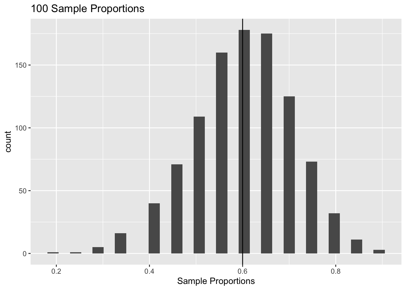
# check parameters
mean(sample_props); p
## [1] 0.59845## [1] 0.6var(sample_props); p * (1 - p) / n## [1] 0.01199709## [1] 0.012Excellent! The sample proportions certainly look bell-curved, and the mean and variance are close to the analytical results that we solved for!
Hopefully this neatly summarizes the basic methodology of inference: parameters, estimators, the whole gamut! We can’t stress enough how important it is to be really comfortable with this stuff, even if it feels really simple. Read it over, and over! Be totally sure!
2.3 Confidence Intervals
In introductory statistics, you may have learned a cookbook method (or formula) for creating confidence intervals, but in this book we will delve deeper mathematically into how they are built. This section will just be a refresher, though; we will get into the intricacies later on.
Confidence Interval for a Mean- You likely know this. It’s a basic form of inference for a parameter, and it’s written in the form:
\[(best \; guess \; \pm \; margin \; of \; error)\]
Say, for example, that you’re interested in estimating the true IQ of college students. Say that your best guess (because of a sample mean, perhaps) is 130. However, you’re obviously not sure if this is exactly right; in fact, you think you’re about 5 points off. Therefore, you might report a confidence interval of \((130 \pm 5) = (125, 135)\), which is basically saying that you’re pretty confident that the true IQ is between 125 and 135 (we’ll formalize “pretty confident” later).
A more telling way to write this general form is:
\[estimate \; \pm \; (z value)(SD \; of \; estimator)\]
Where \(SD \; of \; estimator\) means ‘Standard Deviation of the estimator.’
Now we’re getting to the inference talk. Recall that an estimate is just the specific value that an estimator takes on; the value that the random variable crystallizes to. We know that since the estimator is a random variable, it does indeed have a standard deviation. So, we’re really just centering our confidence interval around our estimate (which we got from our estimator) and we get the width of the interval from the variance of the estimator. This makes sense, because the higher the variance, the wider the interval.
Quick check; why are we multiplying by a z-value? Well, recall the 68-95-99.7 Rule. For a normal distribution, about 68\(\%\) of the data is within 1 standard deviation of the mean, about 95\(\%\) of the data is within 2 standard deviations of the mean, etc. These numbers come from a standard normal \(N(0,1)\), and to translate to a generic normal, \(N(\mu,\sigma^2)\), we simply multiply the standard normal by the standard deviation and add the mean (that is, if \(Z \sim N(0,1)\), then \(\mu + \sigma Z \sim N(\mu, \sigma^2)\)). That’s why we multiply by standard deviations, and why the rule translates into ‘1 standard deviation from the mean, 2 standard deviations from the mean, etc.’; because the base, standard normal has a standard deviation of 1.
These are probably bad explanations, but don’t worry if they don’t make sense to you. Long story short, for a normal distribution, there is a .95 probability of being within 1.96 standard deviations of the mean (remember that we say 95\(\%\) are within about 2 standard deviations of the mean? The true number is 1.96). That’s why we have the CI (confidence interval) set-up that we do.
Let’s write an even more specific example, now: say we want to find a confidence interval for the true population mean. What’s a classic estimator that we might use? Well, we’ve seen that a natural choice is the sample mean, \(\bar{X}\). We know that this is a random variable, and it crystallizes to a specific estimate, \(\bar{x}\). Now say we want a 95\(\%\) confidence interval, or an interval that we are \(95\%\) confident the true mean is in. Recall that the appropriate z-value is 1.96, so we’re going to multiply that by the standard deviation of the estimate. Now, what’s the last piece, the standard deviation of the estimate? We’ve already found the sampling distribution of \(\bar{X}\): given the true population mean, \(\mu\), and variance, \(\sigma^2\), we get…
\[\bar{X} \sim N(\mu,\frac{\sigma^2}{n})\]
So, and let’s assume here that we know the population variance \(\sigma^2\), the standard deviation of our estimator is just the square root of the variance, or \(\sqrt{\frac{\sigma^2}{n}} = \frac{\sigma}{\sqrt{n}}\). Our confidence interval, then, becomes something you’ve likely seen before, or:
\[\bar{x} + 1.96(\frac{\sigma}{\sqrt{n}})\]
Again, this is a 95\(\%\) confidence interval for a population mean using the sample mean; if we want a different level of confidence, we have to change the z-value, here 1.96. If we want a confidence interval for a different parameter, we might use a different estimator (here the sample mean).
2.3.1 Confidence Interval for the Mean, Unknown Variance
Ok, so we know the basic set up for a confidence interval. However, you might have noticed we made a pretty big assumption: we’re using \(\frac{\sigma}{\sqrt{n}}\) as the standard deviation for the estimator, which assumes that we know the population variance \(\sigma^2\) (a parameter) and thus can find \(\sigma\).
You can probably see why this is a little funky; we’re trying to estimate the true mean (parameter) with this confidence interval, so why should we assume that we know the true variance of a population? For example, if you’re interested in the average height of college students and want to estimate it, why on earth would you know the exact variance of the population?
This is a caveat that people often ignore. Indeed, sometimes in introductory statistics, problems just give you the population variance; again, this is nor super realistic. Instead, we’re going to have to estimate the true population variance, which is a parameter, just like we would estimate the mean of a population.
So, what estimator are we going to use to estimate the true population standard deviation? Well, when we wanted to estimate the population mean, we took a sample and then found the sample mean as a good estimate. For the true standard deviation, then, let’s just take a sample, find the standard deviation and use that as an estimate for the true standard deviation!
We’ll get into this more later, but it should make good sense now. Sample means estimate the true population mean, and sample standard deviations estimate the true population standard deviations. We usually denote sample means as \(\bar{x}\), and we usually denote sample standard deviations as \(S\) or \(s\) (uppercase or lowercase; apologies if we get sloppy).
So we’re now using the sample standard deviation instead of the population standard deviation, which means we plug in \(S\) for \(\sigma\) in our confidence interval formula. However, we’re going to change one additional part of the formula. Originally, we multiplied the standard deviation by the critical z-value from a Normal distribution. However, now that we’re using the sample standard deviation to estimate the true standard deviation, we have an added level of uncertainty (we’re not sure what the true standard deviation is; we’re only taking a guess). To account for this added level of uncertainty, we use the t-distribution.
You’ve likely seen the t-distribution before. It’s a doppelganger for the Normal: symmetric, bell-shaped, except that the tails are slightly fatter (the distribution is more spread out). This allows for a little more uncertainty; there’s more density farther away from the center of the distribution.
The confidence interval becomes, then:
\[\bar{x} \pm t^*_{df} \frac{S}{\sqrt{n}}\]
Where \(s\) is the sample standard deviation and \(t^*_{df}\) just means the critical value from a t-distribution with \(df = n - 1\) degrees of freedom; \(n\) here is the sample size. You can almost always find these values in one of those tables, and as \(n\) gets large, the critical values approach the critical z-values. Why does that make sense? Well, as \(n\) gets larger, that just means our sample is getting larger and closer to the entire population, which means that the sample standard deviation becomes closer and closer to the true standard deviation, and thus that added level of uncertainty in estimating the true parameter is greatly diminished (so we can use the z-value again).
2.3.2 Confidence Interval for Proportions
We’ve discussed at length confidence intervals for true population means, but should probably also mention confidence intervals for population proportions. Recall an example of a population: maybe the proportion of college students with red hair. We can use a confidence interval, just like we did with population means, to deliver a reasonable potential interval for this proportion.
Recall the basic set-up for a confidence interval:
\[estimate \; \pm \; (z-value)(SD \; of \; estimator)\]
So we need an estimator; that will just be, as mentioned above, the sample proportion. We need that estimator’s standard deviation; recall the sampling distribution of the sample proportion, \(\hat{p}\):
\[\hat{p} \sim N(p, \frac{pq}{n})\]
Which means the standard deviation of \(\hat{p}\) is \(\sqrt{\frac{pq}{n}}\). However, we’re using \(\hat{p}\) to estimate the true population proportion, \(p\), so in our confidence interval we can’t really use \(p\) because we’re tying to find it; this would be like using a word in the definition of that same word. Instead, like with our mean confidence interval for unknown variance, we have to approximate the standard deviation. What’s our best approximation for \(p\)? Well, it’s \(\hat{p}\). So, the approximated standard deviation of our estimator is \(\sqrt{\frac{\hat{p}(1-\hat{p})}{n}}\).
One last thing; technically, we’re using a Normal distribution to approximate a Binomial here, so we have another level of randomness that we’re not totally accounting for. To fix that, we employ something called the continuity correction. This just means extending each side of the interval by \(\frac{.5}{n}\), where \(n\) is the sample size. You can see that as \(n\) gets large, this correction becomes negligible, because the approximation gets better and better. Our final confidence interval, then, is:
\[\hat{p} \pm z*(\sqrt{\frac{\hat{p}(1-\hat{p})}{n}} + \frac{.5}{n})\]
Where \(z\) is the appropriate z-value.
2.4 Introductory Hypothesis Testing
Again, this is likely a concept you have become very familiar with in earlier stat classes. Let’s go over the basics.
Hypothesis testing is pretty much just like it sounds: you form some sort of educated guess about a population, and then collect data to disprove/support your guess. For example, you might form the hypothesis “the average college male is shorter than 6 feet tall,” then collect data to see how feasible this hypothesis is.
Generally, hypothesis testing consists of two hypothesis: the Null Hypothesis, often denoted as \(H_o\), which can be thought of the status quo or the assumed value, and the Alternative Hypothesis, or \(H_A\), which contradicts the null. For example, you might have the null hypothesis that the average college male height is under 6 feet, and the alternative hypothesis follows naturally: the average college male height is 6 feet or more.
Some important subtleties that you might remember from introductory statistics: you are generally trying to reject the null hypothesis, or collect enough evidence that shows that the null hypothesis is probably wrong. You can never accept the null hypothesis, because you can’t feasibly collect all the data points. You can only lack enough evidence to reject it, and thus fail to reject the null.
For example, say that you made the null hypothesis that all dogs have 4 legs. You could never prove this, as showing it with absolute certainty would require finding all the dogs in the universe. However, you could easily reject this hypothesis if you saw one dog that did not have 4 legs (there are indeed plenty of 3 legged dogs out there). If you take a sample of dogs and get all 4-legged dogs, you might not have enough evidence to reject the null; we would say that you failed to reject the null hypothesis that all dogs have 4 legs.
Ok, so we have all this talk about testing hypotheses, but how do we actually conduct the testing? The general idea is that we take some data and see if the results from the data line up with our hypothesis. In the 4-legged dog example, it’s easy to envision taking a sample of dogs and seeing if we have any that violate our null hypothesis (don’t have 4 legs).
Generally, we’re going to test hypotheses with test statistics. These are tools that take samples from the data and measure how far off the observed data is from our null hypothesis. They have the generic formula:
\[Test \; Statistic \; = \; \frac{Observed \; Statistic \; - \; Expected \; Value \; of \; Statistic}{Standard \; Deviation \; of \; Statistic}\]
Wait a minute…this is just subtracting off a mean and dividing by the standard deviation, or exactly the same method we use when we want to convert to a standard normal. What this is giving us, then, is the number of standard deviation away the observed statistic is from the null hypothesis value.
This is probably getting pretty confusing, so let’s do a basic example. Say that you had a null hypothesis that college students on average weigh 135 pounds. The alternative hypothesis, then, is that college students don’t weight 135 pounds on average. What do you do to test this hypothesis? Well, you take a sample and get an average weight of 145 pounds.
Is that enough evidence to overturn your null hypothesis? Well, you’re good statisticians, so you understand that you need some more info here. If the standard deviation of the sample mean is large (AKA, you get a lot of crazy results from your sample) this might not be a lot of evidence against the null. However, if the standard deviation is small (AKA, you consistently get a sample mean of 145) maybe it’s good evidence against the null.
Let’s say here that the standard deviation of the sample mean is 5 pounds. That means that the observed statistic, 145 pounds, is two standard deviations above the hypothesized value, 135 pounds. And hey, look, that’s what the test statistic would give you: \(\frac{145 - 135}{5} = 2\).
As statistics wizards, you know that being 2 standard deviations away is pretty significant, so it seems likely that your null hypothesis is wrong. That’s the idea, then…look at the test statistic, see how extreme it is, and base your decisions from there.
From this test statistic, we could also calculate a p-value, or the probability that you observe this test statistic or a more extreme one. You can think of it as the probability density beyond the test statistic. In our weight example, this would be the probability density for a normal over two standard deviations above the mean, or \(2.28\%\).
Generally, we’re going to make our conclusions about the null hypothesis (in this book) if the p-value is less than .05 (you’ll find that this is generally the standard convention). That is, if, given that the null hypothesis is true, there is less than a \(5\%\) chance of observing the data that we did. If the chance is that low or lower, we reject the null hypothesis at the \(5\%\) level of statistical significance, and say that we have sufficient evidence to believe that the null is not true (so, in our weight example, we got a p-value of about two percent, and thus we would say that we reject the null and are confident that the average weight is not 135). Otherwise, if the p-value is higher than .05, we fail to reject.
2.4.1 Hypothesis Testing for Means
Recall the generic form for a test statistic:
\[Test \; Statistic \; = \; \frac{Observed \; Statistic \; - \; Expected \; Value \; of \; Statistic}{Standard \; Deviation \; of \; Statistic}\]
If we have a hypothesis about a population mean, we’ve already decided that a good estimator (which is also a statistic; remember, all estimators are statistics) for this parameter. Therefore, we’ll use that as our statistic. We already know the expected value and standard deviation. For the latter, recall that we use \(\frac{S}{\sqrt{n}}\), where \(S\) is the sample standard deviation we used to estimate \(\sigma\). The expected value is \(\mu\), or the true population mean. Since we’re making a guess about the true population mean, this guess is the expected value of the sample mean. We often write this as \(\mu_0\). Therefore, our test statistic becomes:
\[\frac{\bar{x} - \mu_0}{\frac{S}{\sqrt{n}}}\]
Recall that we have a little extra uncertainty because we’re approximating \(\sigma\) with \(S\). That means that we’re going to measure this test statistic against the t-distribution with \(df = n -1\) where \(n\) is the number of data points in the sample (fatter tails, more uncertainty) instead of the standard normal.
Last word here: this seems a little strange because we’re leaving in \(\mu\), but remember that we’re testing if \(\mu_0\), or our hypothesized mean, is a reasonably good guess for the true mean, \(\mu\). That’s why it sticks around; it’s not what we’re trying to estimate, but what we’re trying to test.
2.4.2 Hypothesis Testing for Proportions
If we have a solid understanding of the preceding sections, this should almost be automatic. Remember that our estimator for population proportions, \(p\), is the sample proportion, \(\hat{p}\), and the standard deviation of this estimator is \(\sqrt{\frac{pq}{n}}\). Remember that we want to keep \(p\) in the equation as \(p_0\), or our hypothesized guess for the population proportion. So, we would write our test statistic as:
\[\frac{\hat{p}^* - p_0}{\sqrt{\frac{p_0q_0}{n}}}\]
Why did we write \(\hat{p}^*\) instead of \(\hat{p}\)? Well, recall that we’re using the normal distribution to approximate a binomial, so we need the continuity correction again, or adding/subtracting \(\frac{.5}{n}\) to \(\hat{p}\) (you either add or subtract to make it closer to \(p_0\)). Since we made this correction, you can compare the test statistic to a standard normal z-value.
There are some interesting connections between Hypothesis Tests and Confidence intervals: mainly, if they’re testing the same thing, they should agree. This makes sense because we’re using the same estimators and the same standard deviations for the two approaches. We won’t go really deep here on the connections between the two; after you practice for yourself, you’ll see the connections even better.
Most importantly, you probably are noticing that you relied on a couple of equations to do Hypothesis Testing and Confidence Intervals in your introductory statistics course. That’s because we made these blanket assumptions that the sample is representative of the population and, a big one, that the data is nearly Normal. In this book, we’ll see what happens as these assumptions break down. That is, you will have to really understand how to build these inferential tools, and adapt them to novel situations, not just memorize a couple of formulas. What happens when the data is Exponential? Binomial? All good questions that will be answered on the path to Inference.