Chapter 5 Bayesian Inference

5.1 Motivation

We’ve worked mostly with Frequentist approaches thus far; now it’s time to dive into the newer Bayesian approaches that have been sweeping the statistics world in the past decade. These methods are perhaps more intuitive and exciting ways to make even more inferences about parameters that we’re interested in.

5.2 Bayesian Approach

We’ll get to what it actually means to ‘take a Bayesian approach’; for now, lets’ recall Bayes’ Rule, which we learned in probability. It’s generally used when we have two events $A$ and $B$ and want to go back and forth between the conditional probabilities $P(A|B)$ and $P(B|A)$:

\[P(A|B) = \frac{P(B|A)P(A)}{P(B)}\]

This is clearly an equation for probabilities, but, like we’ve seen with other probability formulas, it can be extended to density functions and random variables. For example, if you had r.v.’s $X$ and $Y$ with PDFs $f(x)$ and $f(y)$, you could write:

\[f(x|y) = \frac{f(y|x)f(x)}{f(y)}\]

Now, let’s think about how we can use this in an environment of inference. Remember the MLE approach? We wanted to find the most likely value for the parameter $\theta$ based on all of the data $X_1, X_2,...,X_n$. In this Bayesian approach, we’re going to do something a little bit different.

Instead of finding a specific value (like the ‘most likely value’) for our parameter based on the data, this Bayesian approach is going to allow us to find the distribution of the parameter given the data we observed. That’s right, we’re going to sample some things, and then form a distribution from our unknown parameter. Once we have that distribution, we could do all types of neat calculations with it: find the mean, variance, etc., all valuable things in estimating the parameter.

Before we get too far ahead of ourselves, let’s stick with the idea that we want the distribution of the parameters given the data. What is that in statistical terms? Well, it’s just $f(\theta|X_1,X_2,...X_n)$ where, again, $\theta$ is the set of parameters and $X_1,X_2,...X_n$ is the data. Let’s try and re-write this using Bayes’ Rule:

\[f(\theta|X_1,X_2,...X_n) = \frac{f(X_1,X_2,...X_n|\theta)f(\theta)}{f(X_1,X_2,...X_n)}\]

This is just straight Bayes Rule from above. Let’s break down the different pieces on the right side. First, we’ve got $f(X_1,X_2,...X_n|\theta)$. That’s just the likelihood function we saw earlier in MLE stuff; we’re familiar with that. What about the denominator, the $f(X_1,X_2,...X_n)$? That’s just the joint PDF of the data; if we have i.i.d. data, then this will be the product of all the marginal PDFs (don’t worry about this too much for right now). The most interesting piece on the right side, though, is $f(\theta)$. This is called the prior distribution for our parameter.

Here’s where things get funky. Recall that we mentioned in Bayesian inference, we’re looking for a distribution of a parameter. For example, let’s say you’re interested in the average IQ at some college. A Bayesian might say that, although this is a true parameter, we’re going to assign some randomness to it. Maybe the true average IQ follows a Normal distribution! Then, the Bayesian would take some data (sample some IQs) and then, based on that data, update the distribution of the true average IQ. For example, maybe you took a huge sample and got a sample mean of 145 and a sample variance of 20. It’s likely that your estimated distribution for the true IQ is going to be somewhere close to $N(145,20)$.

However, we need somewhere to start before we update the distribution of our parameter based on our data. We start with the prior; this basically means that we assign a distribution to a parameter that we want to know. It’s kind of like a way of quantifying the randomness. For example, you might want to put a prior on the true proportion of days that you wake up before 9 AM. This is going to be tough to find exactly, of course, but it’s a perfectly good parameter to try to make inferences about. For this exercise of creating a prior, you might first think that you usually wake up before 9 on weekdays but after on weekends. That’s $\frac{5}{7}$ of the time, or $.71$. So, you’re pretty confident that the true proportion is around there, and you might say, for your random variable prior, that the true proportion follows the distribution $Unif(.6,.8)$. You’re not totally sure, but you’re pretty sure it’s around .7, so you give yourself some space on either side and center your distribution around .7.

Pretty neat, right? The next step here would be to actually take a sample of days (look at a bunch of wake-up times) and, using this data, update the distribution of your parameter. For example, say that you noticed you actually wake up pretty late on Monday and Tuesday? Then your uniform would shift to center on a lower proportion, since you’re waking up before 9 AM less of the time.

Finally, for the rest of this chapter, we’re going to call $f(\theta|X_1,X_2,...,X_n)$, the left hand side of the equation all the way up there, the posterior distribution. If you’ve followed along thus far, this should make pretty intuitive sense. We assigned a prior distribution to our parameter, before we saw any of the data, and then, once we actually observed data, we updated our distribution for the parameter and got this posterior distribution. That is, conditioned on our new data $X_1, X_2, ..., X_n$, we update our PDF for $\theta$.

So, now that we’ve gotten a grasp on everything on the right side, let’s re-visit that application of Bayes Rule.

\[f(\theta|X_1,X_2,...X_n) = \frac{f(X_1,X_2,...X_n|\theta)f(\theta)}{f(X_1,X_2,...X_n)}\]

We can actually simplify this a bit more. The whole point of this, remember, is to get an updated distribution for $\theta$, conditioned on the data; that is, the left side of the equation. We know and can find the stuff in the numerator on the left side of the equation: we’ve shown how to find the likelihood in past sections, and $f(\theta)$, the prior, is just the PDF of whatever distribution we assign. However, the denominator seems to be a little tricky.

Thankfully, in this book, we’re not even going to worry about the denominator (pretty sweet, right?). The reason is that the thing on the left side, the posterior distribution, what we’re concerned with, is a function of $\theta$. That is, we’re interested in the distribution of $\theta$, our parameters. The thing in the denominator of the right side is strictly in terms of different $X$’s, since it’s the joint PDF of a bunch of different observations. It has nothing to do with $\theta$; in fact, it’s just a ‘normalizing constant’ (something we multiply by to make something equal to 1) but it doesn’t affect our approach here.

If you’re confused by this, just remember that we’re interested in $\theta$, and that ugly denominator has nothing to do with $\theta$. What we’re going to do, then, is drop the denominator entirely. This messes with the equality of the two sides, of course, but instead of $=$ we’re now going to write $\propto$, which means “proportional to.”

\[f(\theta|X_1,X_2,...X_n) \propto f(X_1,X_2,...X_n|\theta)f(\theta)\]

We can say these two are proportional because all we would have to do to make them equal is multiply the left side by a constant (the one that we took out: $\frac{1}{f(X_1,X_2,...,X_n)}$. It’s considered a constant because we’re worried about $\theta$; the $X$’s are fixed) to make them equal.

That’s it! Using just the likelihood, which you know well, and the prior, which you can make up to suit your fancy, you’ve just created a PDF for your unknown parameter. It’s pretty crazy, and also does not really sink in until you do an example. Let’s try one now.

All right. Let’s say we are interested in the true proportion of people that have read seen the ‘Lord of the Rings’ trilogy. How are we going to take a sample to estimate this proportion? Well, we’re going to go out in the world and ask people if they have seen the entire trilogy. If they have, then it’s plus one to the ‘yes’ pile; otherwise, plus one to the ‘no’ pile.

So what will our $X_1,X_2,...X_n$ be? This is just our data, remember, and every $X_i$ can take on the value 1 if the person has seen the entire trilogy and 0 otherwise. So, what’s the distribution of every $X_i$? Well, it will be $Bern(p)$, since it’s a yes-no choice with a certain probability, where $p$ is the true proportion of people that have seen the trilogy (the parameter we’re interested in).

That means that we already have the likelihood function. That is, we know $f(X_1,X_2,...X_n|\theta)$. Since our only parameter is $p$, then $\theta = p$ here, and thus the likelihood is the joint distribution of all of the $X$’s conditioned on $p$. That’s just the joint distribution of a bunch of $Bern(p)$ i.i.d. random variables (yes, we are making the assumption that each person is independent, which is not a fully valid assumption, but hopefully does not affect our set-up too much)! Let’s write this out. We know that the PDF of one $X_i$ is $p(1-p)$, since that’s just the PDF of a Bernoulli. Let’s multiply all of them, then:

\[f(X_1,X_2,...X_n|\theta) = \prod_{i=1}^n p^{X_i}(1-p)^{1-X_i} = p^{\sum_{i=1}^n X_i}(1-p)^{n - \sum_{i=1}^n X_i}\]

Let’s look at the first step. Does that make sense? Well, yeah, for every $X_i$, if the person says yes, the PDF will collapse to $p$ because the $X_i$ will be 1, and if they say no, the PDF will collapse to $(1-p)$ because $X_i$ will be 0. So the second step is just the big product of all of these separate PDFs. Then, the third step is just simplifying the large product. Remember, $e^ae^b = e^{a+b}$.

So, anyways, we have our likelihood. We need one more thing, then: our prior. What should we use as our prior? A common choice for proportions is a Beta distribution, because it’s flexible and bounded between 0 and 1. Therefore, let’s use the prior $p \sim Beta(a,b)$. Remember, this is just us assigning a distribution based on our personal previous knowledge. You might choose the $a$ and $b$ to be different numbers based on how many people you think have seen the Lord of the Rings movies; here we’ll just use $a$ and $b$ to maintain generality. What’s our prior, $f(p)$ then? It’s just the PDF of a Beta, or:

\[f(p) = \frac{\Gamma(a + b)}{\Gamma(a)\Gamma(b)}p^{a-1}(1-p)^{b-1}\]

So, let’s put it all together. We’re interested in the posterior distribution, right? That’s $f(p|X_1,X_2,...X_n)$. We know the formula for this based on Bayes rule, and we’ve found the appropriate parts above, so we can just write it out:

\[f(p|X_1,X_2,...,X_n) \propto f(X_1,X_2,...,X_n|p)f(p) = p^{\sum_{i=1}^n X_i}(1-p)^{n - \sum_{i=1}^n X_i}\frac{\Gamma(a + b)}{\Gamma(a)\Gamma(b)}p^{a-1}(1-p)^{b-1}\]

Now, remember, we’re ONLY interested in terms that have $p$, our parameter of interest, in then. That’s why we dropped the marginals of the data points and introduced $\propto$ instead of $=$. So, we can actually drop that normalizing constant of the Beta: the $\frac{\Gamma(a + b)}{\Gamma(a)\Gamma(b)}$, because it’s not important to us. This leads to:

\[f(p|X_1,X_2,...X_n) \propto p^{\sum_{i=1}^n X_i}(1-p)^{n - \sum_{i=1}^n X_i}p^{a-1}(1-p)^{b-1}\]

And we can even simplify this further, since we have terms with $p$ as a base and $(1-p)$ as a base. We can add the exponents to get:

\[p^{a - 1 + \sum_{i=1}^n X_i} (1-p)^{b - 1 + n - \sum_{i=1}^n X_i}\]

Ok…well, that’s kind of ugly. Does that look like a PDF that we recognize? Almost. Let’s just rearrange the sums in the exponents:

\[p^{(a + \sum_{i=1}^n X_i) - 1} (1-p)^{(b + n - \sum_{i=1}^n X_i) - 1}\]

Hey now…that looks like the PDF of a Beta! Specifically, a $Beta(a + \sum_{i = 1}^n X_i, b + n - \sum_{i = 1}^n X_i)$ distribution. Yes, we don’t have the normalizing constant (that nasty thing with the $\Gamma$ stuff out front) but remember that’s not important because we’re only dealing with the meat of it, the terms that relate to $p$.

What’s amazing, then, is we have the posterior distribution of the parameter, given the data we observed. We still have to say $\propto$, because we didn’t include the normalizing constants:

\[f(p|X_1,X_2,...,X_n) \propto Beta(a + \sum_{i = 1}^n X_i, b + n - \sum_{i = 1}^n X_i)\]

Still confused? Let’s say that we started out with a $Beta(10,10)$ distribution as our prior, which is mound-shaped and centered around .5; we can plot the density with dbeta here:

x <- seq(from = 0, to = 1, length.out = 1000)
y <- dbeta(x, 10, 10)
data <- data.table(x = x, y = y)
ggplot(data, aes(x = x, y = y)) +
  geom_line() +
  ggtitle("Density of our Prior Beta(10, 10)")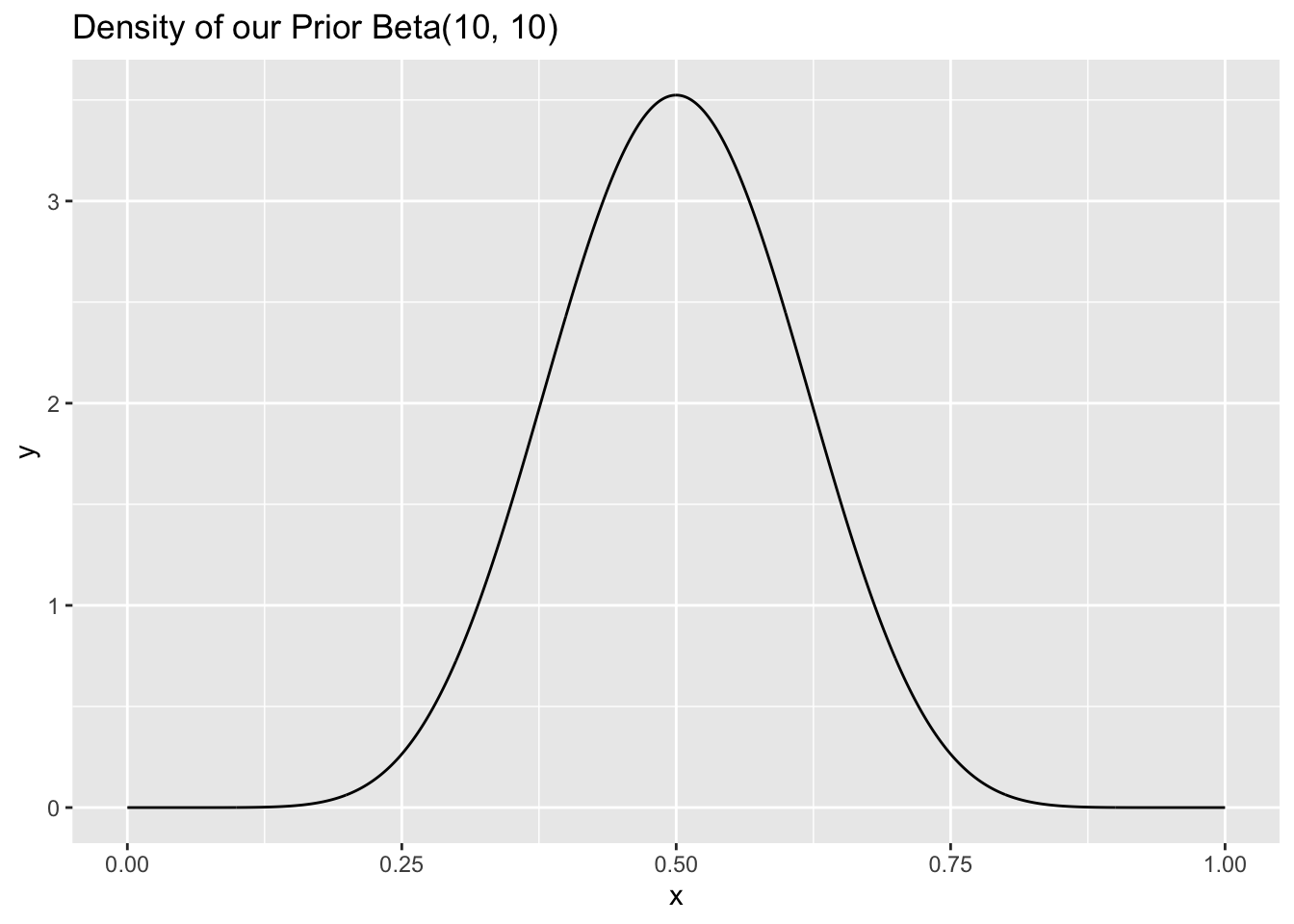

Then we interviewed 100 people, and 70 of them hadn’t seen the trilogy and 30 had. Well, what’s our new distribution for $p$, the parameter? We see above that it’s Beta, with our original $a$ plus the sum of all of the $X_i$’s for the first parameter, and $b + n - \sum_{i = 1}^n X_i$ for the second parameter. Since 30 people said yes, we’re going to add 30 to the original $a$ and 70 (that said no) to the $b$ parameter. The result is a $Beta(10 + 30, 10 + 70)$, or just $Beta(40,80)$ distribution for $p$. Let’s see the density of this posterior distribution:

x <- seq(from = 0, to = 1, length.out = 1000)
y <- dbeta(x, 40, 80)
data <- data.table(x = x, y = y)
ggplot(data, aes(x = x, y = y)) +
  geom_line() +
  ggtitle("Density of our Posterior Beta(40, 80)")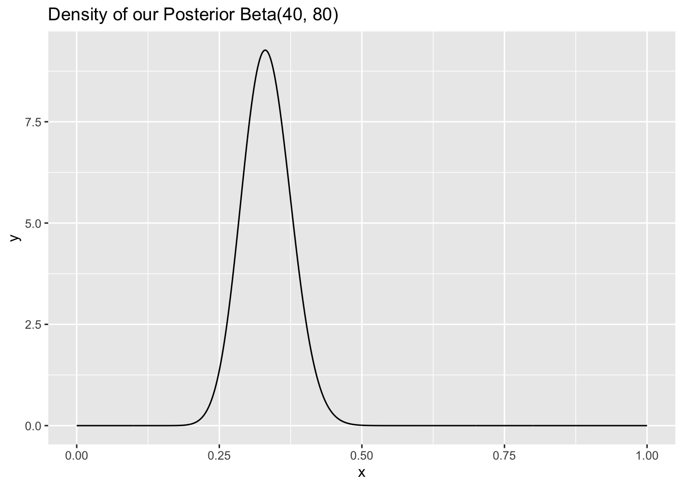

Interestingly, the posterior distribution looks like it is centered closer to $.3$, which makes sense because $30$ of the $100$ people that we sampled had seen the trilogy. That is, the data pushed the distribution, our guess for the parameter, close to the sample proportion. Further, the distribution is less wide; the intuition here is that, now that we have observed more data, we are more confident about the range and values of the parameter $p$.

Hopefully this cleared up some of the questions about the Bayesian approach. This is a pretty neat example because it comes out so cleanly; we start with a Beta and end up with a Beta. This might not happen all the time, so appreciate it when it does! Here are the steps, in general, that you should take for this type of approach.

Find the likelihood, or $f(X_1,X_2,...X_n | \theta)$. Usually this isn’t hard to find, because it’s given.

Find the prior, or $f(\theta)$. Again, this is usually given, or you come up with it yourself.

Multiply (1) and (2) to get the posterior distribution!

Here’s a video version of this walkthrough:

Click here to watch this video in your browser

5.3 Using a Bayesian Approach

Now that we’ve done the major computational part of inference here, let’s talk about smaller, related topics.

5.3.1 Choosing a Prior

The loose definition we used for a prior was a distribution that you think your parameter might reasonably follow. This definitely seems a little bit arbitrary, and really subject to interpretation/whoever is coming up with the distribution. Let’s go over a few good rules of thumb for picking a prior:

Select a prior based on previous data. For example, if you were interested in estimating the true proportion of Harvard students that had ever visited the great state of Connecticut, you might look into the data of how many students traveled to Yale for the most recent playing of their annual football game. Say it was $80\%$ of students. You might reasonably make a prior $Unif(.7,.9)$; that is, centered around .8 but with some uncertainty on either side.

Select an uninformative prior. This would be a prior that provided almost no info, which is helpful because it doesn’t mess with the posterior that much. Imagine if we had made a prior that was totally wrong, and really far off; we would have to collect a lot of data for the ‘ship to right itself’ (the posterior distribution to move away from the incorrect prior distribution and towards the correct true distribution). That’s why using an uninformative prior allows for some flexibility. An uninformative prior for the previous example might be $Unif(0,1)$. It basically gives no information (the proportion can be anywhere from $0$ to $1$), but this lack of specificity might be a good choice if you don’t have any previous data to intelligently form a prior.

Let’s see how, from our above Lord of the Rings example, choosing an uninformative prior $Beta(1, 1)$ instead of $Beta(10, 10)$ changes the posterior distribution (after we observe that 30 out of 100 people have seen the trilogy). We have that a $Beta(1, 1)$ prior is uninformative because it is uniform; it has the same density for any value between $0$ and $1$ (in fact, a $Beta(1, 1)$ is the same as a $Unif(0, 1)$ distribution).

x <- seq(from = 0, to = 1, length.out = 1000)
y <- dbeta(x, 1, 1)
data <- data.table(x = x, y = y)
ggplot(data, aes(x = x, y = y)) +
  geom_line() +
  ggtitle("Density of our Uninformative Prior Beta(1)")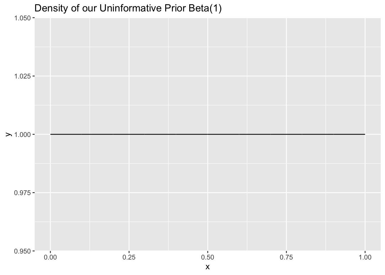

After we observe that 30 people have seen the trilogy and 70 people have not, our posterior distribution becomes $Beta(31, 71)$ (with the same approach from the problem above; just scroll up if you are confused here):

x <- seq(from = 0, to = 1, length.out = 1000)
y <- dbeta(x, 31, 71)
data <- data.table(x = x, y = y)
ggplot(data, aes(x = x, y = y)) +
  geom_line() +
  ggtitle("Density of our Posterior Beta(31, 71)")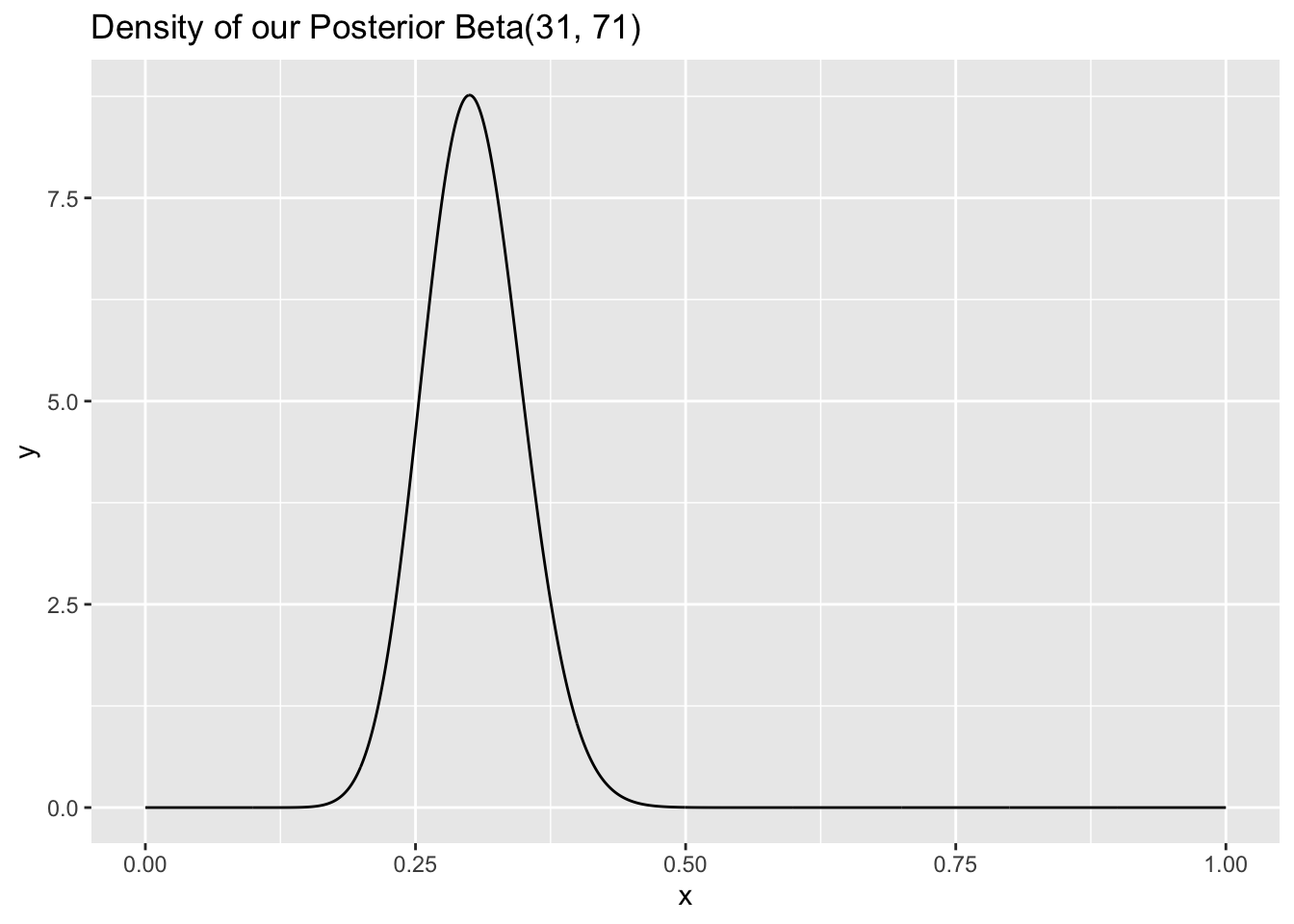

It may be challenging to see, but the ‘mound’ in this density is wider than the $Beta(40, 80)$ density. This might be a desirable characteristic if we are not very confident about the posterior distribution (we will see more about calculating confidence intervals using these distributions soon) and thus we want our posterior distribution to reflect this lack of confidence (i.e., be wider).

Conjugate Priors - These are pretty awesome. Basically, this is when you choose a prior distribution that results in a posterior distribution from the same family. We did an example earlier where we used a Beta prior (for Bernoulli data) and the prior distribution turned into another Beta (updated with the data, but a Beta nonetheless). These are pretty slick, and computationally nice for obvious reasons: you don’t have to code up or learn a new distribution, you can just use the old one!

5.3.2 Bayesian Estimators

So, kind of the whole point of inference is getting estimators for parameters based on the data we observe, right? Well, this section has showed us how to get a distribution for the parameter based on data we observed, but so far there are no estimates to be found. Let’s discuss a couple here.

Bayes Posterior Mean Estimator - This is probably the most intuitive and natural estimator you can get from this approach. Basically, you just take the mean of the posterior distribution you find! For example, if you’re measuring the proportion of redheads at some college and start out with a $Unif(0,.5)$ prior, then, after collecting data, narrow it to $Unif(.2,.3)$, your Posterior Mean estimator would be the mean of this distribution, or .25.

MAP Estimators (Max a Posteriori) - This is the ‘maximum’ of the posterior distribution, or the mode. Same as the mean estimator, but you take the mode of the distribution instead of the mean.

Posterior Median Estimator - You can probably guess what this is: the median of the posterior distribution.

These are all pretty intuitive. They’re basically just summarizing the distribution that you came up with for the unknown parameter.

Loss Functions - We’re not going to go too in depth here, but basically this is a function that measures the error of your estimator. There are tons of different loss functions, because there are tons of different ways to measure error. We’ve already discussed potential Bayesian estimators (posterior mean, median and mode) but you could come up with another estimator based on minimizing a specific loss function.

For example, you could try to minimize how far off your estimator is from the estimate on average. There, the function is distance from the estimate, and we’re finding an estimator by minimizing that difference.

5.4 Bayesian Credible Intervals

This, basically, is a Bayesian version of a Confidence Interval. We try to keep them separate by using words other than ‘confidence’ (belief, credibility, etc), but, make no mistake, it’s pretty much the same thing!

In fact, you might find that these ‘Bayes Credible Intervals’ are more intuitive than most Confidence Intervals you see. Remember that this whole approach centers around the posterior distribution: the distribution of your parameters given the data. If you wanted, say, a $95\%$ confidence interval for one of your parameters, then it makes sense to just report the middle $95\%$ of the posterior distribution.

That is, say you found a posterior distribution for some proportion, and it turned out to be $Unif(.6, .8)$ after observing the data. Then, you could say with $95\%$ belief (remember, we don’t use the word confidence here) that the true proportion is within the interval $(.605, .795)$, or the middle $95\%$ of our interval.

Does that make sense? Hopefully it does. We’re just trying to provide our likely interval that a parameter would live in. We already have this distribution for our parameter that we’ve created, so we mine as well just take the likely interval for that distribution.

You might see this formula for these types of intervals:

\[(q^*_{\frac{\alpha}{2},f(\theta|X_1,X_2,...,X_n)}, q^*_{1 - \frac{\alpha}{2},f(\theta|X_1,X_2,...,X_n)})\]

Let’s break this down. First, let’s talk about the $\frac{\alpha}{2}$ business. Usually, we’re working with $\alpha = .05$, or $1- .05 = .95$ level of confidence (you’ve probably seen this before, this is just notation. We divide by $2$ to account for both sides of the distribution). The $q^*$ things represent quantiles of the distribution. What is a quantile? It’s the value of a distribution, given some ‘percentile in that distribution.’ What does that mean? Well, the $95^{th}$ quantile of a Standard Uniform, $Unif(0,1)$, is the $95^{th}$ percentile of that distribution, or $.95$. If we wanted the $95^{th}$ quantile of a $Unif(0,2)$, that would just be $1.9$ or $2 \cdot .95$.

You can see why this is valuable for these types of intervals. If we want the middle $95\%$ of the data, we just need everything between the $2.5^{th}$ quantile and the $97.5^{th}$ quantile. (since $97.5 - 2.5 = 95$). That’s exactly what we’re doing here; $q^*$ stands for a quantile, so $q^*_{\frac{\alpha}{2}}$ stands for the $2.5^{th}$ quantile and $q^*_{1 - \frac{\alpha}{2}}$ stands for the $97.5^{th}$ quantile when $\alpha = .05$ as it generally does.

We’ve got one more piece to this puzzle, and that’s the $f(\theta|X_1,X_2,...X_n)$ in the subscript of the $q^*$ terms Well, that’s an easy, one; it just means pull the quantiles off of $f(\theta|X_1,X_2,...X_n)$, or the posterior distribution! If you were given $U \sim Unif(0,1)$, then $q^*_{.4,U}$ is just asking for the $40^{th}$ percentile of the $Unif(0,1)$ distribution (which is, of course, $.4$). So, we just asking for the $2.5^{th}$ and $97.5^{th}$ quantiles of the posterior distribution!

This makes total sense because, again, we’re looking for the middle 95$\%$ of the posterior distribution. Usually, we’ll be able to use R to find the quantiles for nasty distributions - although it’s easy to find the quantiles for a standard normal, I bet you couldn’t do it off the top of your head with a Beta! For example, we had a $Beta(40, 80)$ distribution above; we can easily get the quantiles with qbeta:

qbeta(.025, 40, 80)

## [1] 0.2521507

qbeta(.975, 40, 80)

## [1] 0.4197786

Here, then, our ‘belief interval’ is about $.25$ to $.42$.

5.5 Practice

Let $X_i \sim Geom(p)$ be a sample of i.i.d. random variables from a population for $i = 1, ..., n$.

Recall that $p$ is the probability of success on each trial. Give an uninformative prior for $p$

Solution: We can use $Unif(0,1)$, since this spans the entire interval that a probability can take on ($0$ to $1$) but also doesn’t give us any indication of where on that interval the probability parameter would be (by definition, it’s uniform!).

You’re considering alternative priors for $p$. Which do you prefer: a Normal or Beta prior?

Solution: Beta is the more natural choice, as it is bounded from 0 to 1, like a probability. The Normal covers all real numbers.

Say that you assign a $p \sim Beta(\alpha, \beta)$ prior. Find the posterior distribution.

Solution: We’re looking for $f(p|X)$. This is:

\[f(p|X) \propto f(X|p)f(p)\]

We know $f(p)$, since we assigned a distribution to $p$. That’s just the PDF of a Beta.

We also know that $f(X|p)$ is just the likelihood of the X’s, or just the product of a bunch of i.i.d. Geometric random variables with parameter $p$. We get

\[f(p) \propto p^{\alpha-1}(1-p)^{\beta-1}\]

\[f(X|p) = \prod_{i=1}^n q^{x_i} p = q^{\sum_{i=1}^n x_i} p^n\]

Where $q = 1 - p$.

Notice how we drop the normalizing constant (the $\Gamma$ terms) when writing $f(p)$; these terms don’t vary with our parameter $p$ so we don’t care about them. That’s why we wrote $\propto$ (proportional to) instead of $=$.

Multiplying these yields:

\[p^{\alpha-1}(1-p)^{\beta-1}(1-p)^{\sum_{i=1}^n x_i} p^n = p^{n + \alpha - 1} p^{\beta - 1 + \sum_{i=1}^nx_i} \]

This is proportional to a $Beta(n + \alpha, \beta + \sum_{i=1}^n x_i)$. So, we know our posterior:

\[p|X \sim Beta(n + \alpha, \beta + \sum_{i=1}^n x_i)\]

That is, we update the Beta based on our sample size, and then our Beta based on our $x_i$ values. Remember that $x_i$ is the number of failures before the first success in the $i^th$ trial. This makes sense, because the Beta distribution is more left skewed when $\alpha$ is a lot higher than $\beta$ (higher $p$, since less failures) and vice versa.

Find the posterior mean estimate of $p$.

We just take the mean of this Beta. We get:

\[\frac{\alpha + n}{\alpha + n + \beta + \sum_{i=1}^n X_i}\]

Again, this will be larger if there are less failures (i.e., the sum of the $X_i$ values are small).

Find the MLE for $p$.

Solution: We already wrote the likelihood:

\[f(X|p) = \prod_{i=1}^n q^{x_i} p = q^{\sum_{i=1}^n x_i} p^n\]

Taking the log yields:

\[\sum_{i=1}^n x_i log(q) + nlog(p)\]

We can now derive and set equal to 0; it’s easier if we plug in $1 - p$ for $q$. The derivative is

\[\frac{-\sum_{i=1}^n x_i }{1-p}+ \frac{n}{p} = 0\]

\[\frac{1-p}{p} = \frac{\sum_{i=1}^n x_i }{n}\]

Solving gives:

\[\hat{p_{MLE}} = \frac{1}{\frac{\sum_{i=1}^n X_i}{n} + 1} = \frac{1}{\bar{X} + 1}\]

Does that make sense? Well, $\bar{X}$ is how long it takes on average to succeed. If this is large, then $p$ is probably going to be small, which makes sense in our formula. In fact, we would assume a perfect reciprocal relationship, if we did a First Success distribution. Instead, we shift by 1 here.

We can see if our MLE gets close to our true parameter:

# replicate
set.seed(0)

# generate and calculate MLE
x <- rgeom(100, .3)
1 / (mean(x) + 1)

## [1] 0.3389831

Find the MOM for $p$.

Solution: We have one parameter, so we need one moment.

\[\mu = \frac{1-p}{p}\]

Solving yields:

\[p = \frac{1}{\mu + 1}\]

And plugging in for the sample moment yields:

\[\hat{p_{MOM}} = \frac{1}{\bar{X} + 1}\]

So the MOM is the same as the MLE here.

Write a function in R that takes a vector of data and values for $p$, $\alpha$ and $\beta$ and returns the MLE, the MOM and the posterior mean estimate for $p$.

Solution:

We simply code up our solution from above:

FUN_geom <- function(x, p, a, b){
  
    p_mle <- p_mom <- 1 / (mean(x) + 1)
  
    p_pme <- (a + length(x)) / (a + length(x) + b + sum(x))
    
    return(list(p_mle,p_mom,PME))
}

Write a function that takes a vector of data and a value for $p$ and returns the log likelihood of the Geometric.

Solution:

We simply code up our solution from above:

FUN_geomloglik <- function(x, p){
  return(sum(x) * log(1 - p) + length(x) * log(p))
}

Use the optim function to maximize your log likelihood by taking in 100 random draws from a $Geom(.5)$ random variable; make sure that your answer matches the MLE that you solved above.

Solution:

# replicate
set.seed(0)
x <- rgeom(100,.5)

1 / (mean(x) + 1)

## [1] 0.5714286

optim(par = c(.5), fn = FUN_geomloglik, x = x, control = list(fnscale = -1))

## Warning in optim(par = c(0.5), fn = FUN_geomloglik, x = x, control = list(fnscale = -1)): one-dimensional optimization by Nelder-Mead is unreliable:
## use "Brent" or optimize() directly

## $par
## [1] 0.5713867
## 
## $value
## [1] -119.5089
## 
## $counts
## function gradient 
##       20       NA 
## 
## $convergence
## [1] 0
## 
## $message
## NULL

Remember that we need the fnscale = -1 because by default optim minimizes, and this allows us to maximize instead. We can test to make sure that our result (the $par value) matches our MLE:

# replicate
set.seed(0)

x <- rgeom(100,.5)
1 / (mean(x) + 1)

## [1] 0.5714286

Find Fishers Information for $p$.

Solution: We need to take the derivative of the derivative of the log likelihood. This gives:

\[\frac{\sum_{i=1}^n X_i}{(1-p)^2} - \frac{n}{p^2}\]

Now we take the negative expected value:

\[-E(\frac{\sum_{i=1}^n X_i}{(1-p)^2} - \frac{n}{p^2})\]

We know the expectation of $n$ and $p$ are just themselves ($n$ and $p$) because $n$ is a known constant and $p$ is a parameter. We also know that all $E(X_i)$ should be the same by symmetry, so we have $nE(X_1)$. Since $X_1 \sim Geom(p)$, we know $E(X_1) = \frac{1-p}{p}$. So we can write:

\[\frac{n}{p^2} - \frac{n\frac{1-p}{p}}{(1-p)^2} = \frac{n}{p^2} - \frac{n}{p(1-p)}\]