Chapter 18 Overpass API
You will need to install the following packages for this chapter (run the code):
# install.packages('pacman')
library(pacman)
p_load('tidyverse', 'osmdata', 'sf',
'ggmap', 'osmdata', 'osmdata', 'osmdata', 'ggmap')
18.1 Provided Services/Data
What service/data is provided by the API?
The Overpass API grants access to OpenStreetMap (OSM) data (“Overpass API” (2022)). OpenStreetMap is a project founded in 2004 that aims to create a free, open world map using their own data on streets, buildings, rivers, etc. (“FAQs” (2022)). This differs from Google Maps in that the “raw” geo data is provided, meaning that you can easily contribute to the project and tailor the maps (“FAQs” (2022)). The API thus allows you to select certain parts of the OSM data by entering a specific place or type of objects (“Overpass API” (2022)). Some additional services that utilize the API are (“Overpass API/Applications” (2022)):
- Achavi
- OSM Buildings
- Bicycle features
- CoinMap
- Opening_hours map
18.2 Prerequisites
What’s needed to access the API?
Because the Overpass API is open source, no API key or authentication procedures are needed.
It should be noted that the main API server is limited in terms of data size and rate limits (“Overpass API” (2022)). The size of the data can only be known after completing the respective download. Thus, the general rule-of-thumb is that the API can most efficiently download the data of single geographical regions at a time, and data on country-sized regions should rather be obtained via planet.osm mirrors. Regarding rate limits, ca. 1,000,000 requests are allowed per day, and an even safer option is 10,000 queries or 5 GB max. of downloaded data per day.
18.3 Simple API Call
You can use Overpass Turbo provided by Martin Raifer to test Overpass queries and view them in the interactive map. With the Wizard option, you can simply input the elements you are searching for and the corresponding code will be written and executed for you. For example, the default location of the Overpass Turbo is Rome, and by entering the term “Restaurant” into the Wizard, you will then see the code (displayed below) and map results for restaurants in Rome.
/*
This has been generated by the overpass-turbo wizard.
The original search was:
“restaurant”
*/
[out:json][timeout:25];
// gather results
(
  // query part for: “restaurant”
  node["amenity"="restaurant"]({{bbox}});
  way["amenity"="restaurant"]({{bbox}});
  relation["amenity"="restaurant"]({{bbox}});
);
// print results
out body;
>;
out skel qt;
Or if you are already familiar with the query language, you can write your queries directly in the console. Here you also have the option to load, export, or share your data.
Alternatively, it is recommended to use the Wget program. Click here for further details on how to write short and long queries using https.
18.4 API Access in R
What does a simple API call look like in R?
To access the data in R, the package osmdata is needed. This can be installed and loaded as follows:
#install.packages("tidyverse")
#install.packages("osmdata")
#install.packages("sf")
#install.packages("ggmap")
library(tidyverse)
library(osmdata)
library(sf)
library(ggmap)
API queries via Overpass are made using the opq command. As shown below, the argument bbox needs to be specified. For this, you enter the area you want to analyze. In this case, we want to analyze the area of Mannheim, Germany, so we first want to find out the coordinates. The results of the coordinate shows that the degree of latitude is 49.4874592 and degree of longitude is 8.4660395.
If you are unsure about the coordinates that you need for the call, you can simply enter the place you want to research into the getbb() command. The following code then returns the coordinates that you need for your analyses:
##        min      max
## x  8.41416  8.58999
## y 49.41036 49.59047
Since we are not interested in just one point, but an entire area, we specify with the usage of a vector that entails the minimum and maximum degrees of latitude and longitude. Using the command opq we build an Overpass Query that returns the data needed for the analyses.
For the case of Mannheim, the command looks like this:
# opq(bbox = c(minLongitude , minLatitude , maxLongitude , maxLatitude))
library(osmdata)
Mannheim_data <- opq(bbox = getbb("Mannheim")) # Mannheim, Germany
To make the query, the addition of the command add_osm_feature is necessary. It refers to physical features on the ground (e.g., roads or buildings) using tags attached to its basic data structures. Each tag describes a geographic attribute of the feature shown by the specific node, way, or relation. It builds the basis of all following analyses.
The argument key specifies the primary features that can be analyzed. It can take on the following terms:
- “Aerialway”
- “Aeroway”
- “Amenity”
- “Barrier”
- “Boundary”
- “Building”
- “Craft”
- “Emergency”
- “Geological”
- “Healthcare”
- “Highway”
- “Historic”
- “Landuse”
- “Leisure”
- “Man-made”
- “Military”
- “Natural”
- “Office”
- “Place”
- “Power”
- “Public Transport”
- “Railway”
- “Route”
- “Shop”
- “Sport”
- “Telecom”
- “Tourism”
- “Water”
- “Waterway”
Value is the second argument that needs to be specified. It further defines the feature key and defines the kind of physical feature that is loaded with the key- argument. For example, we could be interested in restaurants in Mannheim. Restaurants are part of the general physical feature amenity. The following code returns all restaurants in Mannheim:
Mannheim_restaurants <- opq(bbox = getbb("Mannheim")) %>%
  add_osm_feature(key = 'amenity', value = "Restaurant")
A list of content is returned. At first glance, this data seems confusing because no single data frame is returned, but we instead receive nested data. However, the list obtained is crucial for further analyses and contains important information. We will transform the data set in the last part of this report and provide further insights into the data structure.
Results can be further filtered by adding another value. If we want to filter and receive Italian restaurants, the value term Italian can be added. Restaurants with Italian in the name are then returned.
Italian_restaurants <- opq(bbox = getbb("Mannheim")) %>%
  add_osm_feature(key = 'amenity', value = "Restaurant") %>%
  add_osm_feature(key = 'name', value = "Italian")
It is important to be aware that different languages may be represented in the data downloaded by the Overpass API. It could be, for instance, that a given Italian restaurant does not entail the English word Italian in its name, but rather the German or Italian terms. One could thus adjust the code in the following way:
Italian_restaurants <- opq(bbox = getbb("Mannheim")) %>%
  add_osm_feature(key = 'amenity', value = "Restaurant") %>%
  add_osm_feature(key = 'name', value = c("Italian", "Italia", "Italien", "Italienisch"))
Or via a longer way:
Italian_restaurants <- opq(bbox = getbb("Mannheim")) %>%
  add_osm_feature(key = 'amenity', value = "Restaurant") %>%
  add_osm_feature(key = 'name', value = "Italian") %>%
  add_osm_feature(key = 'name', value = "Italia") %>%
  add_osm_feature(key = 'name', value = "Italien") %>%
  add_osm_feature(key = 'name', value = "Italienisch")
It is also possible to exclude certain values of a feature. This is done by adding an exclamation mark in front of the value.
Wo_restaurants <- opq(bbox = getbb("Mannheim")) %>%
  add_osm_feature(key = 'amenity', value = "!Restaurant")
Moreover, one can also add and combine several requests. For example, we now search for restaurants and pubs:
Restaurants_pubs <- opq(bbox = getbb("Mannheim")) %>%
  add_osm_feature(key = 'amenity', value = "Restaurant") %>%
  add_osm_feature(key = 'amenity', value = "Pub")
Lastly, there is the option to combine via an OR operator. The following code returns restaurants or pubs:
Restaurants_or_pubs <- opq(bbox = getbb("Mannheim")) %>%
  add_osm_feature(key =  c ("\"amenity\"=\"restaurant\"","\"amenity\"=\"pub\""))
Now that we covered the queries, we need to specify the conversion into either Simple Feature Objects (sf), Spatial Objects (sp), Silicate Objects (sc), or XML data.
Simple Feature and Spatial Objects provide OSM components (points, lines, and polygons). osmdata_sf and osmdata_sq return the same data structure, with the exception that osmdata_sf returns data.frame for the spatial variable osm_lines, while osmdata_sq returns SpaitalLinesDataFrame.
Silicate Objects represent the original OSM hierarchy of nodes, ways, and relations. It can convert between complex data types and is especially useful for exploratory aims. However, one needs to be careful using it.
Finally, XML data can be produced. With the function osmdata_xml, raw data are produced and can be saved in XML format.
We use the SF object function, because there is a preexisting geometry function for using the ggplot2 package.
Using the ggmap package, we can visualize our results. First, we need the background map, which is in our case a map of Mannheim. For this, we use the get_map() function. There are more specifications that one can use with the function; such information can be obtained by searching for the function on R or the internet.
To build the graph, we use the ggmap() function, including the object with our background map. In addition, we specify the points of the restaurants in Mannheim with geom_sf(). The argument inherit.aesneeds to be set to FALSE. Depending on our preferences, we can adjust the following settings: colour fill transparency (alpha) size shape (Royé (2018)).
library(osmdata)
library(ggmap)
#our background map
Mannheim_Map <- get_map(getbb("Mannheim"),maptype = "toner-background")

#final map
ggmap(Mannheim_Map)+
  geom_sf(data=SF_Mannheim$osm_points,
          inherit.aes =FALSE,
          colour="#238443",
          fill="#004529",
          alpha=.5,
          size=4,
          shape=21)+
labs(x="",y="") 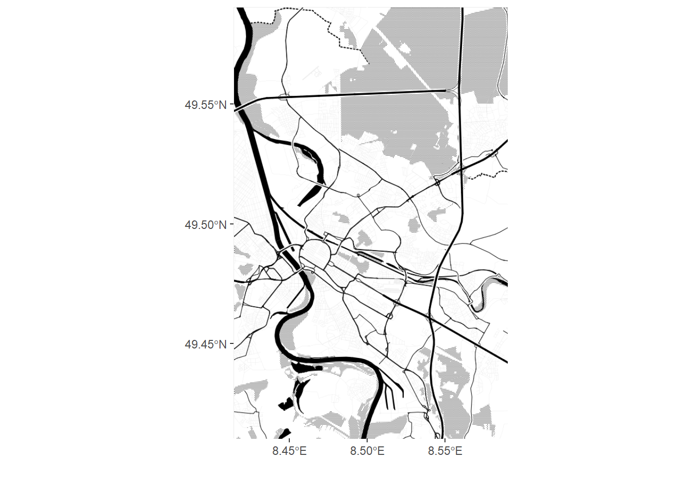
18.5 Social Science Examples
Are there any social science examples using the API?
There is a relatively recent history of utilizing geodata in the social sciences. Ostermann, K. et al. (2022) claimed that today’s spatial research is limited by administrative divisions, e.g., districts and counties. Thus, a major advantage of geodata is its flexibility to be used outside of pre-determined boundaries. Ostermann, K. et al. (2022) applied geodata in labor market research to create a data set of employment biographies of the German working population from 2000 to 2017. They further demonstrated the potential of geodata both on the macro level, such as examining the effect of economic developments on regions, and on the micro scale, for instance determining neighborhood effects and patterns of segregation.
Another line of studies combined geographical information with survey data, such as Hintze and Lakes (2009) who analyzed Germany’s Socio-Economic Panel (SOEP) data. They claimed that adding geodata is beneficial because it provides a complementary source of information, allows for an assessment of spatial patterns and non-spatial variables, and can be transformed into descriptive maps and scatter plots, among others. In the context of the SOEP, they not only used geodata to locating SOEP households but also research the economic and social components of specific areas. Hintze and Lakes (2009) further mentioned the potential of spatial indicators in answering research questions. For instance, households’ accessibility to local infrastructure could be measured by how close homes are to hospitals, schools, public transportation, and cultural infrastructure.
According to Steinberg and Steinberg (2006), geodata and geographic information systems also have potential in policy-based fields, such as: