Data Manipulation
In this chapter, we will learn the most commonly used functions from the dplyr package (and some from the tidyr). The dplyr and tidyr each provides tools to help manipulate and tidy data.
We will use a subset of the 1982 High School & Beyond survey data to demonstrate how to use the functions for data manipulation/transformation. The data set contains ID, minority (0=minority, 1=non-minority), female (0=male, 1=female), SES (socioeconomic status), and mathach (math achievement score) variables for 100 student.
hsb <- read.csv("D://Box Sync/2021 Spring/IntroR_part2/examples/students.csv")  # import data set
str(hsb)   # structure of the data frame
## 'data.frame': 100 obs. of 5 variables:
## $ id : int 1 2 3 4 5 6 7 8 9 10 ...
## $ minority: int 0 0 1 0 1 0 0 0 0 0 ...
## $ female : int 1 1 1 0 1 0 0 0 0 1 ...
## $ ses : num -0.478 1.082 -0.898 0.442 -0.028 ...
## $ mathach : num 3.75 20.69 5.98 24.99 7.03 ...hsb$minority <- as.factor(hsb$minority) # convert 'minority' into a factor
hsb$female <- as.factor(hsb$female) # convert 'female' into a factor
str(hsb) # structure of the data frame## 'data.frame': 100 obs. of 5 variables:
## $ id : int 1 2 3 4 5 6 7 8 9 10 ...
## $ minority: Factor w/ 2 levels "0","1": 1 1 2 1 2 1 1 1 1 1 ...
## $ female : Factor w/ 2 levels "0","1": 2 2 2 1 2 1 1 1 1 2 ...
## $ ses : num -0.478 1.082 -0.898 0.442 -0.028 ...
## $ mathach : num 3.75 20.69 5.98 24.99 7.03 ...Subsetting Data
We have already learned how to subset data using base functions in R (i.e., subset(), squared brackets, …) in the previous video. This chapter will teach you how to subset data in a more straightforward way by using functions from the dplyr package.
Subset Columns
We can select variables (columns) in a data frame using dplyr::select() function. The first argument would be the name of the data frame object, and subsequent arguments are expressions indicating which columns to select.
## select(data, variable_name 1, variable_name 2, variable_name 3, ...)
subset1 <- select(hsb, ses, mathach)  # select 'ses' and 'mathach' variables (columns)
head(subset1)
## ses mathach
## 1 -0.478 3.745
## 2 1.082 20.690
## 3 -0.898 5.982
## 4 0.442 24.993
## 5 -0.028 7.031
## 6 0.852 22.183## select(data, variable_index 1, variable_index 2, variable_index 3, ...)
subset2 <- select(hsb, 3, 5) # select 3rd and 5th variables
head(subset2)## female mathach
## 1 1 3.745
## 2 1 20.690
## 3 1 5.982
## 4 0 24.993
## 5 1 7.031
## 6 0 22.183## Use (:) operator to select a range of consecutive variables
subset3 <- select(hsb, minority:ses) # select a range of variables (from 'minority' to 'ses')
head(subset3)## minority female ses
## 1 0 1 -0.478
## 2 0 1 1.082
## 3 1 1 -0.898
## 4 0 0 0.442
## 5 1 1 -0.028
## 6 0 0 0.852subset4 <- select(hsb, 3:5) # select columns 3-5
head(subset4)## female ses mathach
## 1 1 -0.478 3.745
## 2 1 1.082 20.690
## 3 1 -0.898 5.982
## 4 0 0.442 24.993
## 5 1 -0.028 7.031
## 6 0 0.852 22.183We can also hide variables or take the complement of a set of variables:
## Use (-) or (!) to hide particular variable(s)
subset5 <- select(hsb, -id, -female) # hide 'id' and 'female' variables
head(subset5)
## minority ses mathach
## 1 0 -0.478 3.745
## 2 0 1.082 20.690
## 3 1 -0.898 5.982
## 4 0 0.442 24.993
## 5 1 -0.028 7.031
## 6 0 0.852 22.183subset6 <- select(hsb, !c(id, female)) # select all variables but 'id' and 'female'
head(subset6)## minority ses mathach
## 1 0 -0.478 3.745
## 2 0 1.082 20.690
## 3 1 -0.898 5.982
## 4 0 0.442 24.993
## 5 1 -0.028 7.031
## 6 0 0.852 22.183Subset Rows
We can select rows (observations) based on specific conditions/criteria using dplyr::filter() function. The first argument would be the name of the data frame object, and subsequent arguments are condition statements for filtering data.
## filter(data, condition 1, condition 2, ...)
subset7 <- filter(hsb, female==1) # select rows with 'female = 1'
head(subset7)
## id minority female ses mathach
## 1 1 0 1 -0.478 3.745
## 2 2 0 1 1.082 20.690
## 3 3 1 1 -0.898 5.982
## 4 5 1 1 -0.028 7.031
## 5 10 0 1 0.462 18.831
## 6 14 0 1 0.802 16.387subset8 <- filter(hsb, female==1, mathach > 20) # select rows with 'female = 1' AND 'mathach > 20'
head(subset8)## id minority female ses mathach
## 1 2 0 1 1.082 20.690
## 2 16 1 1 -1.808 22.731
## 3 18 0 1 0.382 23.126
## 4 25 0 1 0.152 22.781
## 5 27 0 1 0.132 21.468
## 6 38 1 1 0.162 20.116We can also use logical operators when multiple conditions are used.
subset9 <- filter(hsb, female==1 & mathach > 20) # select rows with 'female = 1' AND 'mathach > 20'
head(subset9)
## id minority female ses mathach
## 1 2 0 1 1.082 20.690
## 2 16 1 1 -1.808 22.731
## 3 18 0 1 0.382 23.126
## 4 25 0 1 0.152 22.781
## 5 27 0 1 0.132 21.468
## 6 38 1 1 0.162 20.116subset10 <- filter(hsb, female==1 | mathach > 20) # select rows with 'female = 1' OR 'mathach > 20'
head(subset10)## id minority female ses mathach
## 1 1 0 1 -0.478 3.745
## 2 2 0 1 1.082 20.690
## 3 3 1 1 -0.898 5.982
## 4 4 0 0 0.442 24.993
## 5 5 1 1 -0.028 7.031
## 6 6 0 0 0.852 22.183Sort Data
We can use dplyr::arrange() function to sort rows by the values of selected variables. The data is sorted in ascending order by default. To sort the variable(s) in descending order, use desc().
## arrange(data, variable 1, variable 2, .... )
sorted1 <- arrange(hsb, ses)  # reorder rows by 'ses' in ASCENDING order
head(sorted1)
## id minority female ses mathach
## 1 88 1 0 -2.108 -2.262
## 2 92 0 1 -1.878 6.055
## 3 16 1 1 -1.808 22.731
## 4 23 0 1 -1.688 12.825
## 5 58 1 1 -1.578 -2.832
## 6 89 0 1 -1.448 5.122sorted2 <- arrange(hsb, ses, mathach) # reorder rows by 'ses' and 'mathach' in ASCENDING order
head(sorted2)## id minority female ses mathach
## 1 88 1 0 -2.108 -2.262
## 2 92 0 1 -1.878 6.055
## 3 16 1 1 -1.808 22.731
## 4 23 0 1 -1.688 12.825
## 5 58 1 1 -1.578 -2.832
## 6 89 0 1 -1.448 5.122## To sort rows in descending order, use desc()
sorted3 <- arrange(hsb, desc(ses)) # reorder rows by 'ses' in DESCENDING order
head(sorted3)## id minority female ses mathach
## 1 50 0 1 1.512 8.075
## 2 21 0 0 1.332 18.092
## 3 96 0 1 1.302 24.479
## 4 42 0 1 1.282 14.311
## 5 43 0 0 1.262 9.411
## 6 2 0 1 1.082 20.690## or a minus sign
sorted4 <- arrange(hsb, -ses)
head(sorted4)## id minority female ses mathach
## 1 50 0 1 1.512 8.075
## 2 21 0 0 1.332 18.092
## 3 96 0 1 1.302 24.479
## 4 42 0 1 1.282 14.311
## 5 43 0 0 1.262 9.411
## 6 2 0 1 1.082 20.690Add/Modify Columns
To create/add new columns (variables), use dplyr::mutate() or dplyr::transmute(). mutate() adds new variables preserving existing ones; transmute() creates new variables and drops existing ones.
## mutate(data, new_var_name = new_var_values)
# Add 'mathach_std (standardized mathach)' to the data frame
data2 <- mutate(hsb, mathach_std = (mathach - mean(mathach))/sd(mathach))
head(data2)
## id minority female ses mathach mathach_std
## 1 1 0 1 -0.478 3.745 -1.4296013
## 2 2 0 1 1.082 20.690 1.1108467
## 3 3 1 1 -0.898 5.982 -1.0942232
## 4 4 0 0 0.442 24.993 1.7559660
## 5 5 1 1 -0.028 7.031 -0.9369538
## 6 6 0 0 0.852 22.183 1.3346820# Create 'mathach_std' and drop the existing variables
data3 <- transmute(hsb, mathach_std = (mathach - mean(mathach))/sd(mathach))
head(data3)## mathach_std
## 1 -1.4296013
## 2 1.1108467
## 3 -1.0942232
## 4 1.7559660
## 5 -0.9369538
## 6 1.3346820## We can also use operators to create a variable
# 'fem.minority' is TRUE if minority AND female
data4 <- mutate(hsb, fem.minority = minority ==1 & female ==1)
head(data4)## id minority female ses mathach fem.minority
## 1 1 0 1 -0.478 3.745 FALSE
## 2 2 0 1 1.082 20.690 FALSE
## 3 3 1 1 -0.898 5.982 TRUE
## 4 4 0 0 0.442 24.993 FALSE
## 5 5 1 1 -0.028 7.031 TRUE
## 6 6 0 0 0.852 22.183 FALSEWe can remove or modify existing variables as well.
# Modify 'mathach' variable to standardized values
data5 <- mutate(hsb, mathach = (mathach - mean(mathach))/sd(mathach))
head(data5)
## id minority female ses mathach
## 1 1 0 1 -0.478 -1.4296013
## 2 2 0 1 1.082 1.1108467
## 3 3 1 1 -0.898 -1.0942232
## 4 4 0 0 0.442 1.7559660
## 5 5 1 1 -0.028 -0.9369538
## 6 6 0 0 0.852 1.3346820# Remove 'id' and 'minority'
data6 <- mutate(hsb, id=NULL, minority=NULL)
head(data6)## female ses mathach
## 1 1 -0.478 3.745
## 2 1 1.082 20.690
## 3 1 -0.898 5.982
## 4 0 0.442 24.993
## 5 1 -0.028 7.031
## 6 0 0.852 22.183To rename a variable/column, use dplyr::rename() function.
## rename(data, new_var_name = old_var_name)
data7 <- rename(hsb, gender = female) # rename 'female' to 'gender'
head(data7)
## id minority gender ses mathach
## 1 1 0 1 -0.478 3.745
## 2 2 0 1 1.082 20.690
## 3 3 1 1 -0.898 5.982
## 4 4 0 0 0.442 24.993
## 5 5 1 1 -0.028 7.031
## 6 6 0 0 0.852 22.183Summarize Data
In this section, we will cover dplyr::summarise() and dplyr::group_by() which are useful to get summary statistics for grouped/ungrouped data.
To compute summary statistics for ungrouped data, simply use summarise(). The following code produces the mean and standard deviation of SES variable as well as the total number of observations (n() is used to count the number of observations). Note that other functions such as median(), min(), max(), var() can also be applied.
## summarise(data, col_name1 = function1, col_name2 = function2, ...)
summarise(hsb, ses_avrg = mean(ses), ses_sd = sd(ses), n=n())
## ses_avrg ses_sd n
## 1 -0.0213 0.7625503 100To get summary statistics for each group within the data, use group_by() function in addition to summarise(). For example:
## group_by(data, grouping var1, grouping var2, ...)

## Group by one variable
data_grp <- group_by(hsb, female) # Group data by 'female' variable
summarise(data_grp, n=n(), ses_avrg = mean(ses), math_avrg = mean(mathach))
## # A tibble: 2 x 4
## female n ses_avrg math_avrg
## * <fct> <int> <dbl> <dbl>
## 1 0 42 0.0382 14.0
## 2 1 58 -0.0644 12.8## Group by multiple variables
data_grp2 <- group_by(hsb, female, minority) # Group data by 'female' and 'minority'
summarise(data_grp2, n=n(), ses_avrg = mean(ses), math_avrg = mean(mathach))## `summarise()` has grouped output by 'female'. You can override using the `.groups` argument.## # A tibble: 4 x 5
## # Groups: female [2]
## female minority n ses_avrg math_avrg
## <fct> <fct> <int> <dbl> <dbl>
## 1 0 0 33 0.171 15.1
## 2 0 1 9 -0.449 9.80
## 3 1 0 45 0.0776 13.9
## 4 1 1 13 -0.556 8.71Another way to combine multiple functions together is to use the pipe operator: %>%. In this way, we can avoid creating intermediate objects like data_grp in the above example. We can re-write the example code above using the pipe %>% :
hsb %>%
  group_by(female) %>%
  summarise(n=n(), ses_avrg = mean(ses), math_avrg = mean(mathach))
## # A tibble: 2 x 4
## female n ses_avrg math_avrg
## * <fct> <int> <dbl> <dbl>
## 1 0 42 0.0382 14.0
## 2 1 58 -0.0644 12.8hsb %>%
group_by(female, minority) %>%
summarise(n=n(), ses_avrg = mean(ses), math_avrg = mean(mathach))## `summarise()` has grouped output by 'female'. You can override using the `.groups` argument.## # A tibble: 4 x 5
## # Groups: female [2]
## female minority n ses_avrg math_avrg
## <fct> <fct> <int> <dbl> <dbl>
## 1 0 0 33 0.171 15.1
## 2 0 1 9 -0.449 9.80
## 3 1 0 45 0.0776 13.9
## 4 1 1 13 -0.556 8.71summarise() can also be combined with filter(), to summarize data for a specific group.
hsb %>%
  filter(female==1) %>%
  summarise(n=n(), ses_avrg = mean(ses), math_avrg = mean(mathach))
## n ses_avrg math_avrg
## 1 58 -0.06437931 12.75724Reshape/Pivot Data
- Wide format vs. Long format data
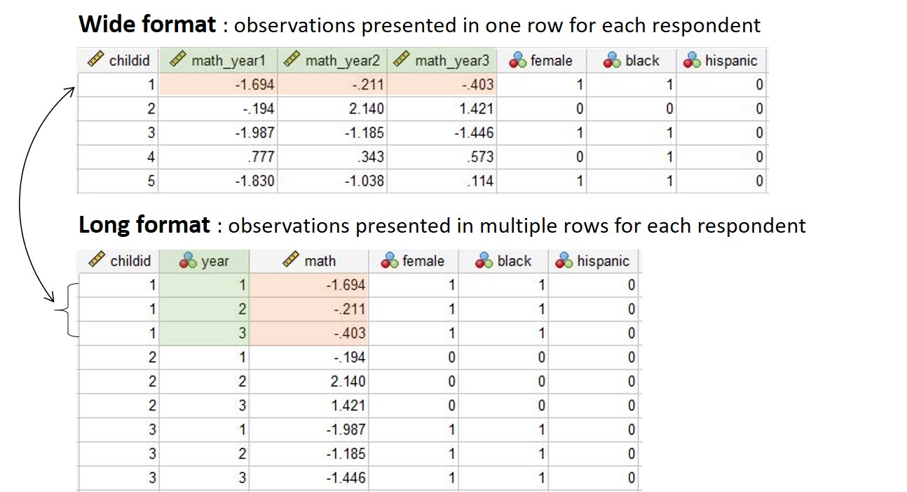 In this section, we will use a different data set (which is longitudinal) to demonstrate how to reshape/pivot data. The data set contains students’ math scores collected for three consecutive years as well as their demographic variables.
threeyrs <- read.csv("D://Box Sync/2021 Spring/IntroR_part2/examples/longitudinal.csv")  # import data set
head(threeyrs)  # print the first 6 rows of the data
## childid math_year1 math_year2 math_year3 female black hispanic
## 1 1 -1.694 -0.211 -0.403 1 1 0
## 2 2 -0.194 2.140 1.421 0 0 0
## 3 3 -1.987 -1.185 -1.446 1 1 0
## 4 4 0.777 0.343 0.573 0 1 0
## 5 5 -1.830 -1.038 0.114 1 1 0
## 6 6 -2.413 -1.694 -1.446 1 1 0- Wide to Long
The original data is in a wide format. To reshape the data to a long format, use tidyr::pivot_longer(). pivot_longer() increases the number of rows and decreases the number of columns.
## pivot_longer(data, columns_to_pivot, names_to = colname_varname, values_to = colname_values)
long <- threeyrs %>%
  pivot_longer(math_year1:math_year3, names_to = "year", values_to = "math")
head(long)
## # A tibble: 6 x 6
## childid female black hispanic year math
## <int> <int> <int> <int> <chr> <dbl>
## 1 1 1 1 0 math_year1 -1.69
## 2 1 1 1 0 math_year2 -0.211
## 3 1 1 1 0 math_year3 -0.403
## 4 2 0 0 0 math_year1 -0.194
## 5 2 0 0 0 math_year2 2.14
## 6 2 0 0 0 math_year3 1.42# Remove prefix of variable names
long2 <- threeyrs %>%
pivot_longer(math_year1:math_year3, names_to = "year", values_to = "math",
names_prefix="math_year", names_transform = list(year = as.integer))
head(long2)## # A tibble: 6 x 6
## childid female black hispanic year math
## <int> <int> <int> <int> <int> <dbl>
## 1 1 1 1 0 1 -1.69
## 2 1 1 1 0 2 -0.211
## 3 1 1 1 0 3 -0.403
## 4 2 0 0 0 1 -0.194
## 5 2 0 0 0 2 2.14
## 6 2 0 0 0 3 1.42- Long to Wide
tidyr::pivot_wider() reshapes the data from long to wide. The function increases the number of columns and decreases the number of rows.
## pivot_wider(data, names_from = colname_varname, values_from = colname_values)
wide <- long2 %>%
  pivot_wider(names_from = "year", values_from = "math")
head(wide)
## # A tibble: 6 x 7
## childid female black hispanic `1` `2` `3`
## <int> <int> <int> <int> <dbl> <dbl> <dbl>
## 1 1 1 1 0 -1.69 -0.211 -0.403
## 2 2 0 0 0 -0.194 2.14 1.42
## 3 3 1 1 0 -1.99 -1.18 -1.45
## 4 4 0 1 0 0.777 0.343 0.573
## 5 5 1 1 0 -1.83 -1.04 0.114
## 6 6 1 1 0 -2.41 -1.69 -1.45# Add prefix to variable names
wide2 <- long2 %>%
pivot_wider(names_from = "year", values_from = "math",
names_prefix="math_year")
head(wide2)## # A tibble: 6 x 7
## childid female black hispanic math_year1 math_year2 math_year3
## <int> <int> <int> <int> <dbl> <dbl> <dbl>
## 1 1 1 1 0 -1.69 -0.211 -0.403
## 2 2 0 0 0 -0.194 2.14 1.42
## 3 3 1 1 0 -1.99 -1.18 -1.45
## 4 4 0 1 0 0.777 0.343 0.573
## 5 5 1 1 0 -1.83 -1.04 0.114
## 6 6 1 1 0 -2.41 -1.69 -1.45Resources
Manuals for dplyr: https://cloud.r-project.org/web/packages/dplyr/dplyr.pdf tidyr: https://cloud.r-project.org/web/packages/tidyr/tidyr.pdf
Datanovia - Data manipulation in R https://www.datanovia.com/en/courses/data-manipulation-in-r/
R for Data Science https://r4ds.had.co.nz/transform.html
IntelliPaat - R tutorial https://intellipaat.com/blog/tutorial/r-programming/data-manipulation-in-r/
Introduction to Data Science by Rafael A. Irizarry https://rafalab.github.io/dsbook/tidyverse.html#manipulating-data-frames