Chapter 2 Basics about Forward and Options
We will explain here the basics about options: definitions and a quick review of Black-Scholes model.
2.1 Risk-Neutral Pricing
The simplest and most basic way to price a derivative that we will study is the following : - Choose a model to diffuse the underlying (and sometimes other parameters) - Use Monte-Carlo method : generate a big number of paths, and compute the discounted expectation (“=”average) of the payoffs for each path.
2.2 Black-Scholes Model
Black-Scholes model is the most common model to diffuse the spot. The formula is described below:
\[ \boxed{dS_t = \mu S_t dt + \sigma dW_t}, \] where \(\mu\) is called the drift, and \(\sigma\) is the implied volatility. A few comments about the model :
The model assumes that the underlying asset follows geometric Brownian motion, which means that the logarithm of the asset’s price changes over time with a constant drift and volatility.
The drift term represents the average rate of return of the underlying asset and is denoted by the symbol \(\mu\). It is typically estimated using historical data or implied from the market.
The volatility, denoted by the symbol \(\sigma\), measures the standard deviation of the asset’s price returns over a specific period. It quantifies the degree of fluctuation or uncertainty in the asset’s price.
The Black-Scholes Model makes several key assumptions:
Risk-Free Interest Rate: The risk-free interest rate, \(r\), is constant and known. This is used in discounting the expected payoff at maturity.
European Options: The model assumes European options which can only be exercised at expiration.
No Dividends: During the life of the option, the underlying asset does not pay a dividend.
No Arbitrage: There are no opportunities to make a risk-free profit (i.e., arbitrage opportunities do not exist).
Log-Normal Distribution: The returns on the underlying asset are normally distributed, which implies that the asset prices are log-normally distributed. The density function for a log-normal distribution is given by \(f(x) = \frac{1}{x\sigma \sqrt{2\pi}} e^{-(\log x - \mu)^2 / (2\sigma^2)}\) for \(x > 0\).
Frictionless Markets: Trading in the market is costless, and there are no restrictions on borrowing or short selling.
2.3 Forward contract
- A forward contract gives the buyer the obligation to buy a stock S at a pre-determined price K (the strike) at a horizon of time T (maturity).
- Forward contracts are trader Over-The-Counter (OTC), whereas Futures are standardized contracts traded on the market. By a non-arbitrage argument, we find the price of a forward :
\[ \boxed{\text{Forward}_t(T) = (F_t(T)-K)e^{-r(T-t)}} \]
We can derive the forward price, which will be very important for after :
\[ \boxed{\text{F}_t(T) = S_0e^{(r-q+repo)T}} \]
- When the dividends increase, the forward decreases: by a non-arbitrage argument, when the dividend is detached, the stock should decrease of the value of the dividend, otherwise we could buy the stock, earn the dividend and sell the stock. The profit would be the dividend, and there would be no risk.
- When the repo rate increases, the forward increases: by a non-arbitrage argument, when the repo rate rises, borrowing shares for short selling becomes more expensive. If the forward price doesn’t increase, we could borrow money at the repo rate, buy the stock, and sell at the unchanged forward price, making a risk-free profit.
Why is this value so important ? When pricing options and estimating values, the forward is the reference value of the stock in the future.
2.4 Calls and Put options
- A Call option is a contract that allows the buyer to buy a stock S at a pre-determined level K (the strike), at a horizon of time T (maturity).
\[ \boxed{\text{Payoff}=(S_T - K)^+} \] The graph of the payoff is the following:
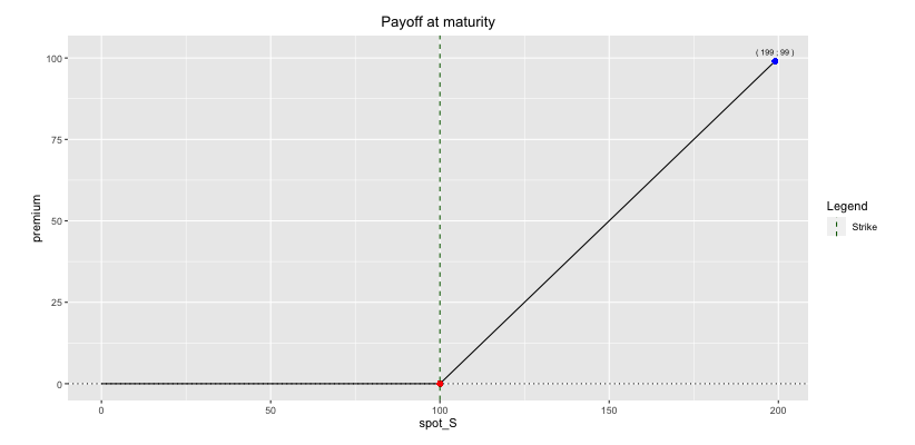
Call Option Payoff
- A Put option is a contract that allows the buyer to sell a stock S at a pre-determined level K (the strike), at a horizon of time T (maturity). \[ \boxed{\text{Payoff}=(K-S_T)^+} \] The graph of the payoff is the following:
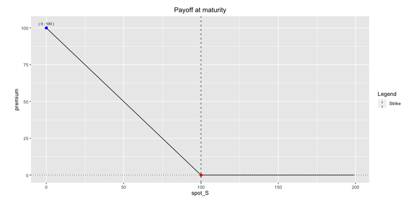
Put Option Payoff
2.4.1 Call Put parity
Before deriving the prices of the two above instruments, the call-put parity defines the relation between the price of the Call and the price of the Put: \[ \boxed{C-P = S_T - Ke^{-(r-q)(T-t)}} \] This result can be interpreted graphically by combining the two graphs above. ## Option pricing