Chapter 7 Case Study

library(tidyverse)
library(survival)
library(survminer)
library(gtsummary)
library(scales)

The guidelines for reporting the Kaplan-Meier test are from Laerd’s Kaplan-Meier using SPSS Statistics (Laerd 2015). The data is from survival::lung.

d_lung <- survival::lung %>%
  filter(!is.na(ph.ecog)) %>%
  mutate(
    ph.ecog = factor(
      ph.ecog,
      levels = c(0, 1, 2, 3, 4),
      labels = c("Asymptomatic", "Ambulatory", "In bed <50%", "In bed >50%", "Bedridden")),
    ph.ecog = fct_drop(ph.ecog),
    ph.ecog = fct_lump_n(ph.ecog, n = 2, other_level = "Bedridden"),
    patient_id = row_number()
  )

A study investigated differences in all-cause mortality between men and women diagnosed with advanced lung cancer. 227 participants aged 39 to 82 were monitored up to three years until time of death. The participants were segmented into three groups according to their ECOG performance score: asymptomatic, symptomatic but completely ambulatory, and bedridden at least part of the day. Participant age was captured as a controlling covariate.

(t1 <- d_lung %>%
  mutate(status = factor(status, levels = c(1, 2), labels = c("censored", "died"))) %>%
  tbl_summary(by = "ph.ecog", include = c(time, status, ph.ecog, age)) %>%
  add_overall())

Characteristic	Overall, N = 227¹	Asymptomatic, N = 63¹	Ambulatory, N = 113¹	Bedridden, N = 51¹
time	259 (168, 399)	303 (224, 438)	243 (177, 426)	180 (100, 301)
status
censored	63 (28%)	26 (41%)	31 (27%)	6 (12%)
died	164 (72%)	37 (59%)	82 (73%)	45 (88%)
age	63 (56, 69)	61 (56, 68)	63 (55, 68)	68 (60, 73)
¹ Median (IQR); n (%)

7.1 Cox

The Cox proportional hazards model describes the effect of explanatory variables on survival and can include controlling variables. Add age as a controlling variable.

cox_fit <- coxph(Surv(time, status) ~ ph.ecog + age, data = d_lung)
(cox_tbl <- cox_fit %>% gtsummary::tbl_regression(exponentiate = TRUE))

Characteristic	HR¹	95% CI¹	p-value
ph.ecog
Asymptomatic	—	—
Ambulatory	1.43	0.97, 2.11	0.072
Bedridden	2.39	1.52, 3.74	<0.001
age	1.01	0.99, 1.03	0.2
¹ HR = Hazard Ratio, CI = Confidence Interval

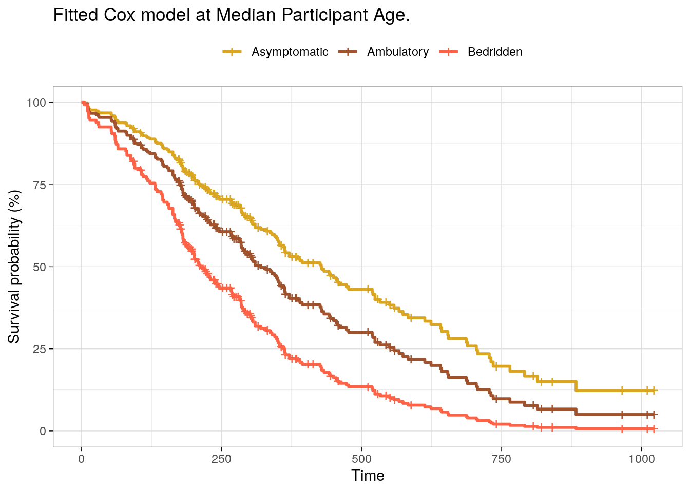
Using a Cox proportional hazards regression analysis, we find the association between ECOG and survival time statistically significant with a Bedridden estimate of 2.39 (95% CI 1.52, 3.74; p<0.001) relative to Asymptomatic. The hazard ratio for Ambulatory was not statistically significant, 1.43 (95% CI 0.97, 2.11; p=0.072).

survfit(cox_fit, newdata = list(ph.ecog = levels(d_lung$ph.ecog),
                                             age = rep(median(d_lung$age), 3)), data = d_lung) %>%
  surv_summary() %>%
  ggsurvplot_df(
    fun = "pct",
    # linetype = "strata", # Change line type by groups
    # conf.int = TRUE,
    surv.median.line = "hv", # median horizontal and vertical ref lines
    ggtheme = theme_light(),
    palette = c("goldenrod", "sienna", "tomato"),
    title = "Fitted Cox model at Median Participant Age.",
    legend.title = "",
    legend.labs = levels(d_lung$ph.ecog)
  )

7.2 Discrete Time

To fit a discrete time model, first create a discrete time data set, on record per relevant time period. You could do this by hand with expand.grid()

cs_glm_dat <- expand.grid(
  time = seq(min(d_lung$time), max(d_lung$time), 1),
  patient_id = unique(d_lung$patient_id)
) %>%
  inner_join(d_lung, by = "patient_id") %>%
  filter(time.x <= time.y) %>%
  mutate(status = if_else(time.x < time.y, 0, status - 1)) %>%
  rename(time = time.x)

But discSurv::dataLong does this for you.

cs_glm_dat <- d_lung %>% 
  mutate(status = status - 1) %>%
  discSurv::dataLong("time", "status", timeAsFactor = FALSE)

For example, patient 1 died at time 306, so they have 306 rows in the new data set, with y = 0 for all but the last row.

cs_glm_dat %>% filter(obj == 1) %>% tail()

##       obj timeInt y inst time status age sex    ph.ecog ph.karno pat.karno
## 1.300   1     301 0    3  306      1  74   1 Ambulatory       90       100
## 1.301   1     302 0    3  306      1  74   1 Ambulatory       90       100
## 1.302   1     303 0    3  306      1  74   1 Ambulatory       90       100
## 1.303   1     304 0    3  306      1  74   1 Ambulatory       90       100
## 1.304   1     305 0    3  306      1  74   1 Ambulatory       90       100
## 1.305   1     306 1    3  306      1  74   1 Ambulatory       90       100
##       meal.cal wt.loss patient_id
## 1.300     1175      NA          1
## 1.301     1175      NA          1
## 1.302     1175      NA          1
## 1.303     1175      NA          1
## 1.304     1175      NA          1
## 1.305     1175      NA          1

glm() fits either the log(-log(1-hazard)) or log(hazard / (1-hazard)) as a function of time, controlling for ph.ecog and age. The two links are similar here⁶.

cs_glm_dat %>%
  group_by(ph.ecog, timeInt) %>%
  summarise(.groups = "drop", died = sum(y), at_risk = n()) %>%
  mutate(
    hazard = died / at_risk,
    logit_hazard = log(hazard / (1 - hazard)),
    cloglog_hazard = log(-log(1 - hazard))
  ) %>%
  pivot_longer(cols = c(logit_hazard, cloglog_hazard)) %>%
  filter(!hazard %in% c(0, 1)) %>%
  ggplot(aes(x = timeInt, y = value, color = ph.ecog)) +
  geom_point() +
  geom_smooth(method = "lm", formula = "y ~ x") +
  facet_wrap(facets = vars(name)) +
  theme_light()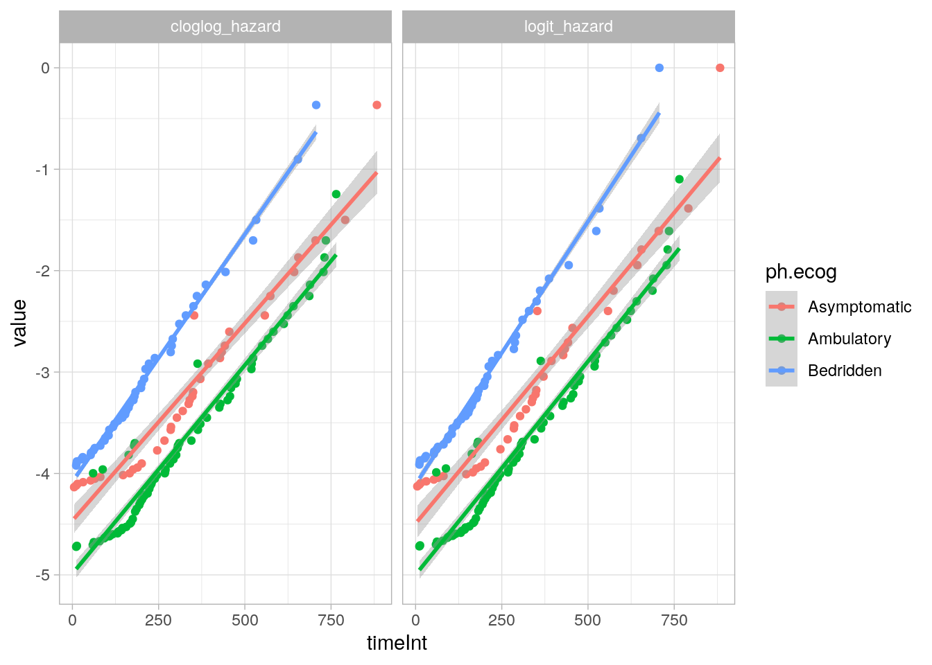

logit_fit <- glm(
  y ~ timeInt + ph.ecog + age, 
  data = cs_glm_dat, 
  family = binomial(link = "logit")
)
(logit_tbl <- logit_fit %>% gtsummary::tbl_regression(exponentiate = TRUE))

Characteristic	OR¹	95% CI¹	p-value
timeInt	1.00	1.00, 1.00	<0.001
ph.ecog
Asymptomatic	—	—
Ambulatory	1.42	0.97, 2.11	0.081
Bedridden	2.38	1.52, 3.76	<0.001
age	1.01	0.99, 1.03	0.3
¹ OR = Odds Ratio, CI = Confidence Interval

Using a discrete time logistic regression analysis with logit link function, we find the association between ECOG and survival time statistically significant with a Bedridden estimate of 2.38 (95% CI 1.52, 3.76; p<0.001) relative to Asymptomatic. The hazard odds ratio for Ambulatory was not statistically significant, 1.42 (95% CI 0.97, 2.11; p=0.081).

cloglog_fit <- glm(
  y ~ timeInt + ph.ecog + age, 
  data = cs_glm_dat, 
  family = binomial(link = "cloglog")
)
(cloglog_tbl <- cloglog_fit %>% gtsummary::tbl_regression(exponentiate = TRUE))

Characteristic	HR¹	95% CI¹	p-value
timeInt	1.00	1.00, 1.00	<0.001
ph.ecog
Asymptomatic	—	—
Ambulatory	1.41	0.97, 2.11	0.081
Bedridden	2.38	1.52, 3.75	<0.001
age	1.01	0.99, 1.03	0.3
¹ HR = Hazard Ratio, CI = Confidence Interval

Using a discrete time logistic regression analysis with complementary log-log link function, we find the association between ECOG and survival time statistically significant with a Bedridden estimate of 2.38 (95% CI 1.52, 3.75; p<0.001) relative to Asymptomatic. The hazard ratio for Ambulatory was not statistically significant, 1.41 (95% CI 0.97, 2.11; p=0.081).

7.3 Reporting

The reporting below uses the Cox model rather than the discrete time model.

Participants were randomly assigned to three different interventions in order to quit smoking: a hypnotherapy programme (n = 50), wearing nicotine patches (n = 50) and using e-cigarettes (n = 50). Kaplan-Meier survival analysis (Kaplan & Meier, 1958) was conducted to compare the three different interventions for their effectiveness in preventing smoking resumption. A similar percentage of censored cases was present in the hypnotherapy (12.0%), nicotine patch (14.0%) and e-cigarette (14.0%) intervention groups and the pattern of censoring was similar. Participants that underwent the hypnotherapy programme had a median time to smoking resumption of 69.0 (95% CI, 45.2 to 92.8) days. This was longer than the groups receiving nicotine patches or e-cigarettes, which had identical median times to smoking resumption of 9.0 (95% CI, 6.6 to 11.4) days and 9.0 (95% CI, 7.1 to 10.9) days, respectively. A log rank test was conducted to determine if there were differences in the survival distributions for the different types of intervention. The survival distributions for the three interventions were statistically significantly different, χ2(2) = 25.818, p < .0005. Pairwise log rank comparisons were conducted to determine which intervention groups had different survival distributions. A Bonferroni correction was made with statistical significance accepted at the p < .0167 level. There was a statistically significant difference in survival distributions for the hypnotherapy vs nicotine patch intervention, χ2(1) = 11.035, p = .001, and hypnotherapy vs e-cigarette intervention, χ2(1) = 29.003, p < .0005. However, the survival distributions for the e-cigarette and nicotine patch interventions were not statistically significantly different, χ2(1) = 1.541, p = .214.

References

Laerd. 2015. Statistical Tutorials and Software Guides. https://statistics.laerd.com/.

Full discussion on Rens van de Schoot.↩︎