Chapter 2 Survey Design
The survey design (aka, sampling strategy), ultimately depends on how study objective(s) are translated into survey questions, the units of analysis of the target population, the main variables and covariates, and the available sampling frame(s) for data collection (Valliant 2013). Exploratory surveys often sample individuals with qualifying characteristics by convenience, snowball (referrals), quota, or purposeful sampling (Lau 2017). In contrast to these non-probability sampling strategies, descriptive and explanatory surveys use probability sampling, including simple random sapling (SRS) and stratified sampling.4 Whichever survey design you use, you will employ one of three criteria to determine the sample size: i) set a target coefficient of variation, \(CV_0(\theta) = SE / \theta\); ii) set a target \(SE\); or iii) set a target margin of error (aka, tolerance), \(MOE = \pm z_{1-\alpha} \cdot SE\).
2.1 Simple Random Sampling
Suppose you have simple random sample (SRS) of size \(n\) from a population of size \(N\). The estimated population parameters is \(\bar{y}_U\) with variance \(S^2\). The sample mean, \(\bar{y}_s\), is the expected value of \(\bar{y}_U\). Under repeated sampling, the sample means would differ with variance
\[ \begin{equation} V(\bar{y}_s) = \left(1 - \frac{n}{N} \right) \frac{S^2}{n}. \tag{2.1} \end{equation} \]
Equation (2.1) is square of the familiar formula for the standard error of the estimate, \(SE(\bar{y}_s) = S / \sqrt{n}\), multiplied by the finite population correction factor (FPC), \(1 - n / N\). The FPC reduces the expected variance for finite (small) populations. The ratio of the corrected \(SE\) and \(\bar{y}_U\) is called the coefficient of variation, CV. You’ll often see it expressed as its square, \(CV^2(\bar{y}_s) = V(\bar{y}_s) / \bar{y}_U^2\),
\[ \begin{equation} CV^2(\bar{y}_s) = \left(1 - \frac{n}{N} \right) \cdot \frac{1}{n} \cdot \frac{S^2}{\bar{y}_U^2}. \tag{2.2} \end{equation} \]
The final term, \(\frac{S^2}{\bar{y}_U^2}\) is the square of the unit CV (aka population CV),
\[ \begin{equation} CV(\bar{y}_U) = \frac{S}{\bar{y}_U} \tag{2.3} \end{equation} \]
Solve Equation (2.3) for \(n = \frac{S^2 / \bar{y}^2_U}{CV_0^2 + S^2 / (N \cdot \bar{y}^2_U)}\) to establish the minimum sample size required to achieve a targeted CV, \(CV_0(\bar{y}_s)\). Function PracTools::nCont() does the calculation for you, but you need to supply values for the targeted CV and unit CV. Setting the unit CV is somewhat of a chicken-and-egg problem since \(S^2\) and \(\bar{y}_U^2\) are the population parameters you are estimating in the first place. You’ll have to rely either on prior research or your best guess. The range rule of thumb, \(S = \mathrm{range} / 4\), is a useful tool for \(S^2\). The targeted CV is usually set to match or beat prior research, or is set arbitrarily. Values of 5% and 10% are common.
Example. Suppose from prior experience you think the unit CV is \(CV(\bar{y}_U) = 2\). You desire a targeted CV of \(CV_0(\bar{y}_s) = 0.10\).
CV0 <- .10
CVpop <- 2
PracTools::nCont(CV0 = CV0, CVpop = CVpop) %>% ceiling()
## [1] 400

# Notice N was not specified. You only need to worry about N if it is small. If
# you don't know CVpop or ybarU and S2, but at least have an expectation about
# ybarU and the range of values, try the range rule of thumb.
my_ybarU <- 100
my_S <- abs(0 - 800) / 4
my_S^2
## [1] 40000
(my_CVpop <- my_S^2 / my_ybarU)
## [1] 400
PracTools::nCont(CV0 = CV0, S2 = my_S^2, ybarU = my_ybarU) %>% ceiling()
## [1] 400

# When does N become important? It depends on CV0. N=20,000 seems to be upper limit.
expand.grid(
  CV0 = c(.05, .10),
  N = c(5E4, 4E4, 3E4, 2E4, 1E4, 5E3, 4E3, 3E3, 2E3, 1E3, 500, 400, 300, 200, 100)
) %>%
  mutate(n = map2_dbl(CV0, N, ~PracTools::nCont(CV0 = .x, CVpop = CVpop, N = .y))) %>%
  ggplot(aes(x = N, y = n, color = as.factor(CV0))) +
  geom_line() +
  # geom_vline(aes(xintercept = 5000), linetype = 3, color = "#00BFC4") +
  geom_segment(aes(x = 5000, xend = 5000, y = 0, yend = 400),
               linetype = 3, color = "#00BFC4", linewidth = 1) +
  geom_segment(aes(x = 0, xend = 5000, y = 400, yend = 400),
               linetype = 3, color = "#00BFC4", linewidth = 1) +
  geom_segment(aes(x = 0, xend = 20000, y = 1500, yend = 1500),
               linetype = 3, color = "#F8766D", linewidth = 1) +
  geom_segment(aes(x = 20000, xend = 20000, y = 0, yend = 1500),
               linetype = 3, color = "#F8766D", linewidth = 1) +
  labs(color = "CV0")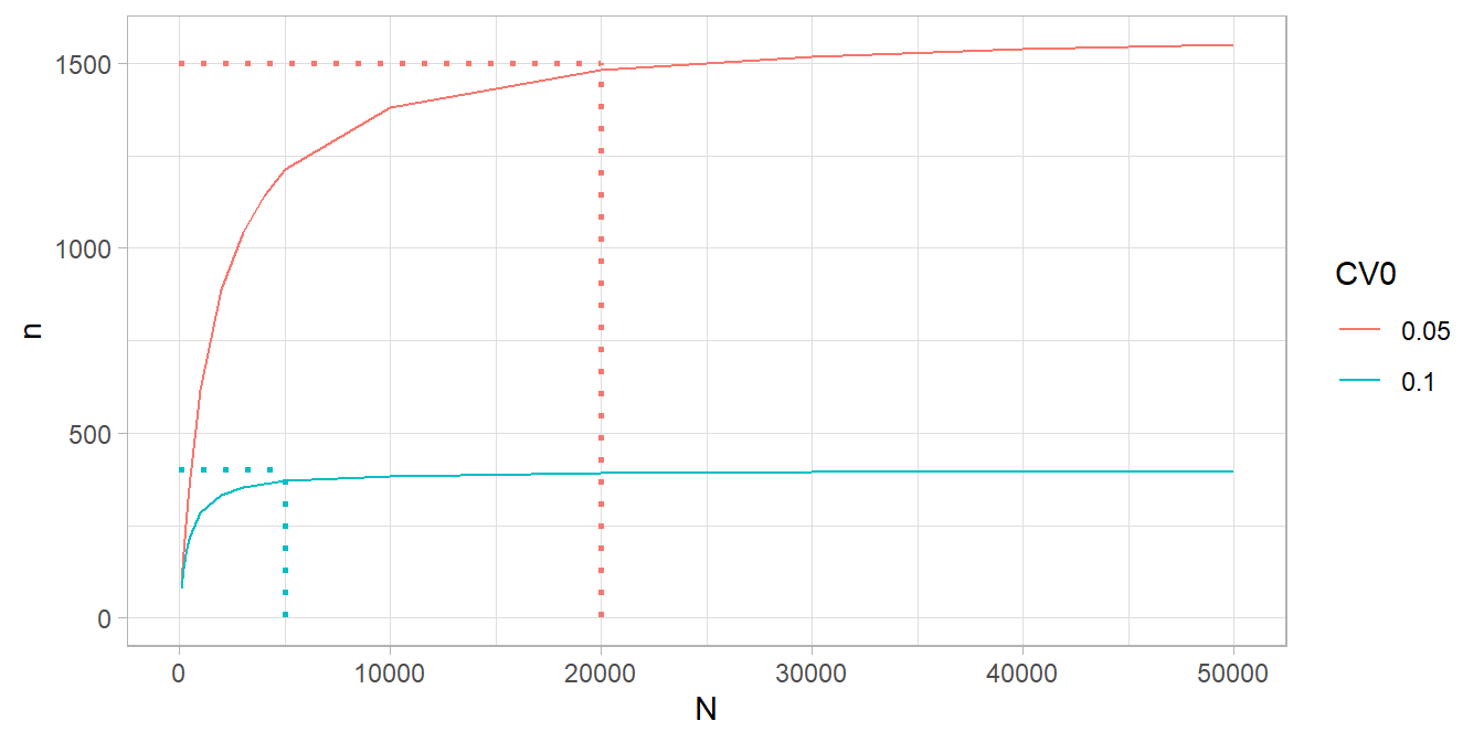
If the population parameter is a proportion, \(p_U\), the CV is
\[ \begin{equation} CV^2(p_s) = \left(1 - \frac{n}{N} \right) \cdot \frac{1}{n} \cdot \frac{N}{N-1} \cdot \frac{1 - p_U}{p_U} \tag{2.4} \end{equation} \]
where \(\frac{N}{N-1} \cdot \frac{1 - p_U}{p_U}\) is the square of the unit CV. When \(N\) is large, Equation (2.4) reduces to \(CV^2(p_s) \approx \frac{1}{n} \cdot \frac{1 - p_U}{p_U}\). From here you can see that \(n\) varies inversely with \(p_U\). Function PracTools::nProp() calculates \(n\) for proportions.
Example. Suppose from prior experience you think \(p_U = .01\) and the \(N\) is large. You set a targeted CV of \(CV_0^2(p_s) = 0.05\).
CV0 <- .05
pU <- .01
N <- Inf
PracTools::nProp(CV0 = CV0, pU = pU, N = N)
## [1] 39600
Whoa, \(n\) was huge! You might choose to target a margin of error instead, \(MOE = \pm z_{1-\alpha} \cdot SE\). Recall that \(P(|p_s - p_U| < MOE) = 1 - \alpha\). PracTools::nPropMoe() and PracTools::nContMoe() calculate \(n\) for MOEs.
Example. Continuing from above, suppose you set a tolerance of a half percentage point, \(MOE \pm 0.5\%\).
MOE <- .005
# moe.sw = 1 sets MOE based on SE; moe.sw = 2 sets MOE based on CV.
PracTools::nPropMoe(moe.sw = 1, e = MOE, alpha = .05, pU = pU, N = N)
## [1] 1521.218

# The long way using nProp:
(z_025 <- qnorm(p = .05/2, lower.tail = FALSE))
## [1] 1.959964
(SE <- MOE / z_025)
## [1] 0.002551067
PracTools::nProp(V0 = SE^2, N = N, pU = pU)
## [1] 1521.218

# When pU is extreme (~0 or ~1), the 95% CI can pass the [0,1] limits. The Wilson
# method accounts for that (not discussed here). Notice the 95% CI is not symmetric
# about pU. The 95% CI calculation is one of the reasons it is used.
PracTools::nWilson(moe.sw = 1, e = MOE, alpha = .05, pU = pU)
## $n.sam
## [1] 1605.443
##
## $`CI lower limit`
## [1] 0.00616966
##
## $`CI upper limit`
## [1] 0.01616966
##
## $`length of CI`
## [1] 0.01

# The log odds is another approach that does about the same thing.
PracTools::nLogOdds(moe.sw = 1, e = MOE, alpha = .05, pU = pU, N = N)
## [1] 1637.399
2.2 Stratified SRS
Stratified samples partition the population by dimensions of interest before sampling. This way, important domains are assured of adequate representation. Stratifying often reduce variances. Choose stratification if i) an SRS risks poor distribution across the population, ii) you have domains you will study separately, or iii) there are units with similar mean and variances that can be grouped to increase efficiency.
In a stratified design, the measured mean or proportion of the population is the simple weighted sum of the \(h\) strata, \(\bar{y}_{st} = \sum{W_h}\bar{y}_{sh}\) and \(p_{st} = \sum{W_h}p_{sh}\). The population sampling variance is analogous,
\[ \begin{equation} V(\bar{y}_{st}) = \sum W_h^2 \cdot \left(1 - \frac{n_h}{N} \right) \cdot \frac{1}{n_h} \cdot S_h^2. \tag{2.5} \end{equation} \]
Use the SRS sampling methods described in Section 2.1 to estimate each stratum.
Example. Suppose you are measuring expenditure within a company of \(N = 875\) employees and want to stratify by the \(h = 6\) departments. You target a \(CV_0(\bar{y_s}) = .10.\)
data(smho98, package = "PracTools")

# You'll survey 560 people across the 16 strata.
smho98 %>%
  group_by(STRATUM) %>%
  summarize(Nh = n(), Mh = mean(EXPTOTAL), Sh = sd(EXPTOTAL)) %>%
  mutate(
    CVpop = Sh / Mh,
    nh = map2_dbl(CVpop, Nh, ~PracTools::nCont(CV0 = .10, CVpop = .x, N = .y) %>% ceiling())
  ) %>%
  janitor::adorn_totals("row", fill = NULL, na.rm = FALSE, name = "Total", Nh, nh)
##  STRATUM  Nh         Mh         Sh     CVpop  nh
##        1 151 13066021.0 14792181.7 1.1321107  70
##        2  64 40526852.3 37126887.6 0.9161059  37
##        3  43 11206761.2 11531709.1 1.0289957  31
##        4  22  7714828.7  8422580.5 1.0917391  19
##        5 150  4504517.9  6228212.0 1.3826589  85
##        6  23  2938983.2  3530750.8 1.2013511  20
##        7  65  7207527.1  9097011.5 1.2621543  47
##        8  14  1879611.1  1912347.8 1.0174168  13
##        9  38 13841123.7 11609453.3 0.8387652  25
##       10  12  5867993.8  6427340.3 1.0953216  11
##       11  13   925512.8   659352.8 0.7124189  11
##       12  77  4740554.8  6905571.9 1.4567012  57
##       13  59  9060838.1 12884439.0 1.4219920  46
##       14  86  9511349.0  6741831.0 0.7088196  32
##       15  39 34251923.7 82591916.4 2.4113074  37
##       16  19  4629061.5  9817393.7 2.1208173  19
##    Total 875         NA         NA        NA 560

# What if we don't stratify? Only 290!
smho98 %>%
  summarize(Nh = n(), Mh = mean(EXPTOTAL), Sh = sd(EXPTOTAL)) %>%
  mutate(
    CVpop = Sh / Mh,
    nh = map2_dbl(CVpop, Nh, ~PracTools::nCont(CV0 = .10, CVpop = .x, N = .y) %>% ceiling())
  ) %>% janitor::as_tabyl()
##   Nh       Mh       Sh    CVpop  nh
##  875 11664181 24276522 2.081288 290
If a fixed budget constrains you to \(n\) participants you have five options: i) if \(S_h\) are approximately equal and you are okay with small stratum getting very few units, allocate \(n\) by proportion, \(n_h = nW_h\); ii) if your strata are study domains, allocate \(n\) equally, \(n_h = n / H\); iii) use Neyman allocation to minimize the population sampling variance; iv) use cost-constrained allocation to minimize cost, or v) use precision-constrained allocation to minimize population sampling variance. Options iv and v take into account variable costs. Use function PracTools::strAlloc().
The Neyman allocation allocates by stratum weight,
\[ \begin{equation} n_h = n \cdot \frac{W_h S_h}{\sum W_h S_h}. \tag{2.6} \end{equation} \]
Suppose your costs vary by stratum, \(c_h\). The cost-constrained allocation starts with \(C = c_0 + \sum n_h c_h.\) Minimizing the population sampling variance,
\[ \begin{equation} n_h = (C - c_0) \frac{W_hS_h / \sqrt{c_h}}{\sum W_h S_h \sqrt{c_h}}. \tag{2.7} \end{equation} \]
This method allocates more population to larger strata and strata with larger variances. The precision-constrained allocation is
\[ \begin{equation} n_h = (W_h S_h / \sqrt{c_h}) \frac{\sum W_h S_h \sqrt{c_h}}{V_0 + N^{-1} \sum W_h S_h^2}. \tag{2.8} \end{equation} \]
Example. Suppose you have a fixed budget of $100,000. If sampling costs are $1,000 person, survey \(n = 100\) people and allocate \(n\) to \(n_h\) with options i-iii). If sampling costs vary by stratum, use options iv-v).
# Stratum per capita survey costs
ch <- c(1400, 400, 300, 600, 450, 1000, 950, 250, 350, 650, 450, 950, 80, 70, 900, 80)

smho98 %>%
  group_by(STRATUM) %>%
  summarize(Nh = n(), Mh = mean(EXPTOTAL), Sh = sd(EXPTOTAL)) %>%
  bind_cols(
    `i) prop` = ceiling(.$Nh / sum(.$Nh) * 100),
    `ii) equal` = ceiling(1 / nrow(.) * 100),
    `iii) neyman` = PracTools::strAlloc(n.tot = 100, Nh = .$Nh, Sh = .$Sh,
                                        alloc = "neyman") %>% pluck("nh") %>% ceiling(),
    ch = ch,
    `iv) cost` = PracTools::strAlloc(Nh = .$Nh, Sh = .$Sh, cost = 100000, ch = ch,
                                     alloc = "totcost") %>% pluck("nh") %>%
      ceiling(),
    `v) prec.` = PracTools::strAlloc(Nh = .$Nh, Sh = .$Sh, CV0 = .10, ch = ch,
                                         ybarU = .$Mh, alloc = "totvar") %>%
      pluck("nh") %>% ceiling()
  ) %>%
  select(-c(Mh, Sh)) %>%
  janitor::adorn_totals("row", fill = NULL, na.rm = FALSE, name = "Total", Nh,
                        `i) prop`, `ii) equal`, `iii) neyman`, `iv) cost`, `v) prec.`)
##  STRATUM  Nh i) prop ii) equal iii) neyman   ch iv) cost v) prec.
##        1 151      18         7          18 1400       19       12
##        2  64       8         7          19  400       37        3
##        3  43       5         7           4  300        9        7
##        4  22       3         7           2  600        3        3
##        5 150      18         7           8  450       14       25
##        6  23       3         7           1 1000        1        2
##        7  65       8         7           5  950        6        8
##        8  14       2         7           1  250        1        2
##        9  38       5         7           4  350        8        5
##       10  12       2         7           1  650        1        2
##       11  13       2         7           1  450        1        1
##       12  77       9         7           5  950        6       10
##       13  59       7         7           6   80       27       26
##       14  86      10         7           5   70       22       20
##       15  39       5         7          26  900       34        4
##       16  19       3         7           2   80        7       12
##    Total 875     108       112         108   NA      196      142
2.3 Power Analysis
Sections 2.1 and 2.2 calculated sample sizes based on the desired precision of the population parameter using CV, MOE, and cost constraints. Another approach is to calculate the sample size required to detect the alternative value in a hypothesis test. Power is a measure of the likelihood of detecting some magnitude difference \(\delta\) between \(H_0\) and \(H_a\).5 Power calculations are best suited for studies that estimate theoretical population values, not for studies that estimate group differences in a finite population (Valliant 2013).
A measured \(t = \frac{\hat{\bar{y}} - \mu_0}{\sqrt{v(\hat{\bar{y}})}}\) test statistic would vary with repeated measurements and have a \(t\) distribution. A complication about the degrees of freedom arises in survey analysis. It is usually defined using a rule of thumb: \(df = n_{psu} - n_{strata}\). So if you have 10 strata and 100 PSUs per stratum, \(df\) would equal 1,000 - 100 = 900.
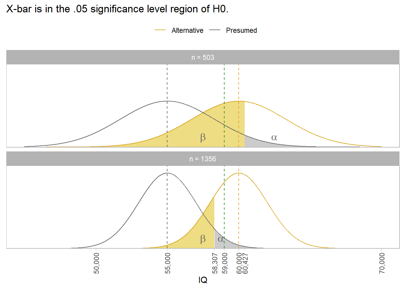
Example. Suppose you want to measure mean household income for married couples. From prior research, you expect the mean is $55,000 with 6% CV. You hypothesize \(\mu\) is greater than $55,000, but only care if the difference is at least $5,000.
The 6% CV implies SE = 6% * $55,000 = $3,300. Supposing \(\sigma\) = $74,000, the original research would have use a sample of size n = \((\$74,000 / \$3,300)^2\) = 503.
Don’t use n = 503 for your sample though. The probability of measuring a sample mean >= $60,000 with an acceptable p-value is the power of the study. For n = 503 the power is only 0.448. The area of 1 - \(\beta\) in the top panel below is only pnorm(qnorm(.95, 50000, 3300), 55000, 3300, lower.tail = FALSE) = 0.448. To achieve a 1-\(\beta\) = .80 power, you need n = 1,356. That’s what the bottom panel shows. Notice that a sample mean of $59,000 still rejects H0: \(\mu\) = $55,000. The power of the test tells you the sample size you need to draw a sample mean large enough to reject H0 1-\(\beta\) percent of the time.
The power of the test from the original study was only 0.448.
power.t.test(
  type = "one.sample",
  n = 503,
  delta = 5000,
  sd = 74000,
  sig.level = .05,
  alternative = "one.sided"
)
##
## One-sample t test power calculation
##
## n = 503
## delta = 5000
## sd = 74000
## sig.level = 0.05
## power = 0.4476846
## alternative = one.sidedWith such a low power of the study, a sample mean of $59,000 isn’t large enough to reject H0. Its p-value would be pt(q = (59000-55000)/(74000/sqrt(503)), df = 503 - 1, lower.tail = FALSE) = 0.113. To find the right sample size, use the power calculation with 1 - \(\beta\) and n unspecified.
power.t.test(
  type = "one.sample",
  delta = 5000,
  sd = 74000,
  sig.level = .05,
  power = .80,
  alternative = "one.sided"
)
##
## One-sample t test power calculation
##
## n = 1355.581
## delta = 5000
## sd = 74000
## sig.level = 0.05
## power = 0.8
## alternative = one.sided2.4 Appendix: Bias
A consideration not explored here, but which should be on your mind is the risk of bias. Here are a few types of bias to beware of (Lau 2017).
- Coverage bias. The sampling frame is not representative of the population. E.g., school club members is a poor sampling frame if target population is high school students.
- Sampling bias. The sample itself is not representative of the population. This occurs when response rates differ, or sub-population sizes differ. Explicitly define the target population and sampling frame, and use systematic sampling methods such as stratified sampling. Adjust analysis and interpretation for response rate differences.
- Non-response bias. Responded have different attributes than non-respondents. You can offer incentives to increase response rate, follow up with non-respondents to find out the reasons for their lack of response, or compare the characteristics of non-respondents with respondents or known external benchmarks for differences.
- Measurement bias. Survey results differ from the population values. The major cause is deficient instrument design due to ambiguous items, unclear instructions, or poor usability. Reduce measurement bias with pretesting or pilot testing of the instrument, and formal tests for validity and reliability.
References
Cluster sampling, systematic sampling and Poisson sampling are other sampling methods to at least be aware of. I’m not ready to deal with these yet.↩︎
See statistics handbook section on frequentist statistics for discussion of Type I and II errors.↩︎