Chapter 5 Results
In examining the total payments exchanged each year, there is an obvious difference in the scale of the 2015-2019 data and the 2020 data. While the 2015-2019 data is in the hundreds of millions, the 2020 data doesn’t reach $70 million. This could be due to a lag in reporting of payments, or it could reflect decreased transactions due to the COVID-19 pandemic, which began in the US in the first quarter of 2020. Thus, the 2020 data points should be considered with caution.
| Years | Total Payments |
|---|---|
| 2015 | 218,908,281 |
| 2016 | 102,052,022 |
| 2017 | 179,455,555 |
| 2018 | 179,486,553 |
| 2019 | 185,317,184 |
| 2020 | 69,956,239 |
5.1 Payment Characteristics
5.1.1 Type of Payment
Payment types are dominated by 3 types: consulting fees, food and beverage, and compensation for services other than consulting. These payment types are approximately 10 times more expensive than the other categories.
Consulting fees are "payment[s] that a company makes to a physician for advice and expertise about a medical product or treatment (Medicare & Medicaid Services (2022b)). However, this definition is extremely vague and is applied by the pharmaceutical companies themselves. The other two dominating categories have no direct association with medical expertise.
| Nature of Payment | 2015 | 2016 | 2017 | 2018 | 2019 | 2020 |
|---|---|---|---|---|---|---|
| Royalty or License | 12.33 | 6.02 | 5.59 | 8.09 | 9.46 | 26.47 |
| Consulting Fee | 37.57 | 16.58 | 35.10 | 38.83 | 33.87 | 14.86 |
| Food and Beverage | 73.97 | 32.09 | 63.57 | 58.46 | 51.13 | 14.03 |
| Compensation for services other than consulting, including serving as faculty or as a speaker at a venue other than a continuing education program | 56.13 | 24.19 | 45.10 | 46.20 | 60.83 | 7.97 |
| Grant | 5.58 | 4.30 | 4.33 | 4.55 | 3.36 | 2.50 |
| Current or prospective ownership or investment interest | 6.38 | 8.04 | 5.80 | 4.12 | 6.64 | 1.64 |
| Travel and Lodging | 17.89 | 8.81 | 14.56 | 13.75 | 13.64 | 0.95 |
| Honoraria | 3.13 | 0.55 | 1.87 | 1.62 | 1.65 | 0.62 |
| Gift | 0.23 | 0.01 | 0.79 | 1.92 | 2.07 | 0.38 |
| Education | 2.73 | 0.99 | 1.36 | 1.29 | 2.05 | 0.36 |
| Compensation for serving as faculty or as a speaker for a non-accredited and noncertified continuing education program | 2.89 | 0.09 | 1.07 | 0.54 | 0.49 | 0.13 |
| Compensation for serving as faculty or as a speaker for an accredited or certified continuing education program | 0.05 | 0.29 | 0.09 | 0.05 | 0.11 | 0.04 |
| Entertainment | 0.01 | 0.01 | 0.01 | 0.08 | 0.01 | 0.00 |
| Charitable Contribution | 0.01 | 0.08 | 0.22 | 0.01 | 0.01 | 0.00 |
Interestingly, while food and beverage garners huge amounts of funding on the aggregate level, it has the second least expensive average payment. Thus, this payment type must be extremely popular and often used by the pharmaceutical industry to build relationships with primary care physicians.
| Nature of Payment | 2015 | 2016 | 2017 | 2018 | 2019 | 2020 |
|---|---|---|---|---|---|---|
| Royalty or License | 97.83 | 52.82 | 37.29 | 56.58 | 46.81 | 164.42 |
| Current or prospective ownership or investment interest | 193.27 | 423.07 | 290.03 | 216.73 | 255.57 | 126.37 |
| Grant | 7.63 | 10.00 | 9.23 | 9.40 | 5.66 | 7.58 |
| Compensation for serving as faculty or as a speaker for an accredited or certified continuing education program | 2.80 | 3.84 | 3.05 | 3.51 | 2.79 | 2.31 |
| Consulting Fee | 1.40 | 3.77 | 3.02 | 2.93 | 2.77 | 2.31 |
| Compensation for services other than consulting, including serving as faculty or as a speaker at a venue other than a continuing education program | 1.82 | 2.38 | 2.22 | 2.26 | 3.39 | 1.56 |
| Compensation for serving as faculty or as a speaker for a non-accredited and noncertified continuing education program | 2.16 | 2.95 | 1.91 | 2.15 | 2.33 | 1.55 |
| Honoraria | 2.03 | 2.17 | 2.53 | 2.25 | 2.36 | 1.45 |
| Gift | 0.14 | 0.14 | 0.62 | 1.96 | 2.28 | 0.61 |
| Travel and Lodging | 0.40 | 0.39 | 0.35 | 0.33 | 0.35 | 0.27 |
| Education | 0.03 | 0.04 | 0.02 | 0.04 | 0.05 | 0.08 |
| Entertainment | 0.08 | 0.10 | 0.11 | 0.55 | 0.13 | 0.07 |
| Food and Beverage | 0.02 | 0.02 | 0.02 | 0.02 | 0.02 | 0.02 |
| Charitable Contribution | 0.98 | 2.02 | 4.34 | 2.78 | 1.95 | 0.00 |
5.1.2 Population Density
As would be expected, ZIP codes categorized as “Extremely Dense” and “Dense” have the highest amount of both total and average payments, while ZIP codes categorized as “Extremely Sparse” and “Sparse” have the lowest amount of both total and average payments. This makes sense, as dollars would go the furthest when paid to primary care physicians serving ZIP codes with dense populations, as these physicians are seeing and having an impact on the greatest number of patients.
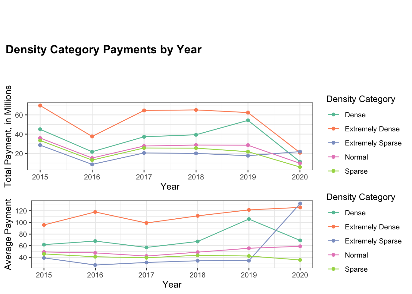
For each year of the study, one-way ANOVA analysis was performed to determine if there was a statistically significant difference in payments to ZIP codes of the 5 different density categories. Each ANOVA returned a p-value of less than \(\alpha < 0.05\), so it seems there is a significant difference between the density categories.
| Years | P-value |
|---|---|
| 2015 | <0.001 * |
| 2016 | <0.001 * |
| 2017 | <0.001 * |
| 2018 | <0.001 * |
| 2019 | <0.001 * |
| 2020 | 0.0414 * |
5.2 Geospatial
5.2.1 ZIP Code
The first level of geospatial analysis considers payments aggregated by ZIP code. The table below shows summary statistics for the top ZIP code (in total payments) for each year. The table highlights the wide range of payments to ZIP codes, with the top ZIP codes in 2019 and 2020 receiving over 15 million dollars, while the top ZIP codes from 2015-2018 are under 6 million dollars.
| Years | Top ZIP Code (total payments) | Total Payments | No. of Payments | No. of Physicians | Avg. Payment | Amount per Physician |
|---|---|---|---|---|---|---|
| 2015 | 75390 | 5,336,835.31 | 679 | 125 | 7,859.85 | 42,694.68 |
| 2016 | 75390 | 5,112,483.24 | 438 | 86 | 11,672.34 | 59,447.48 |
| 2017 | 75390 | 3,300,777.35 | 775 | 140 | 4,259.07 | 23,576.98 |
| 2018 | 55404 | 3,111,817.94 | 89 | 18 | 3,964.25 | 172,878.77 |
| 2019 | 85020 | 18,656,875.69 | 609 | 67 | 30,635.26 | 278,460.83 |
| 2020 | 95966 | 15,826,688.30 | 57 | 13 | 277,661.20 | 1,217,438 |
As the figures further confirm, ZIP code may be too nuanced of a means for comparison, as there are over 40,000 ZIP codes in the USA, and the payments vary widely.
5.2.2 State
Thus, let us compare payments on a state level. For each year, the leading state in total payments was California. This makes sense due to California’s large population. As the table shows, there is less fluctuation year to year on the state level, so this analysis may prove more fruitful.
| Years | Top State (total payments) | Total Payments | No. of Payments | No. of Physicians | Avg. Payment | Amount per Physician |
|---|---|---|---|---|---|---|
| 2015 | California | 35,954,080 | 367,403 | 20,365 | 97.86 | 1,765.48 |
| 2016 | California | 13,997,319.39 | 155,796 | 13,578 | 89.84 | 1,030.88 |
| 2017 | California | 25,073,460 | 324,136 | 19,309 | 77.35 | 1,298.54 |
| 2018 | California | 27,366,160 | 293,444 | 19,513 | 93.26 | 1,402.46 |
| 2019 | California | 25,846,585.07 | 255,469 | 17,793 | 101.17 | 1,452.63 |
| 2020 | California | 21,528,528.10 | 74,094 | 7,304 | 290.56 | 2,947.50 |
Each figure represents the log total payments to the continental US states for the listed year. In observing the changes in colors over the study period, it seems log total payments to primary care physicians in states in the Northeast decreased over time, while log total payments to primary care physicians in states in the West increased.
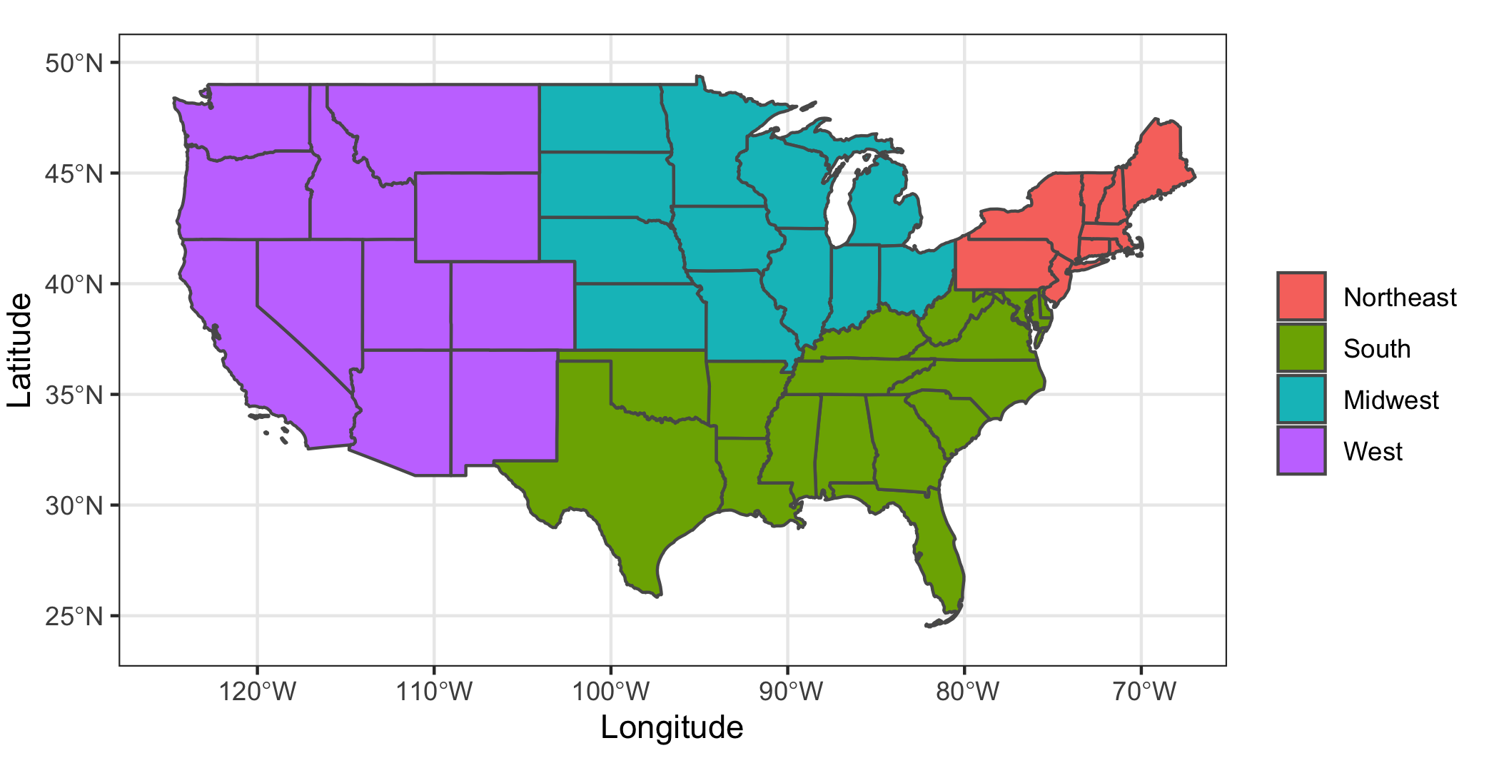
5.2.3 Region
To get a better sense of regional changes in log total payments to primary care physicians, states were grouped into the 4 regions identified below.
The plot of total payments to each region shows that the South received the highest aggregate amount for most of the time period. As anticipated above, primary care physicians in states in the West region saw an increase in aggregate payments, while primary care physicians in states in the Northeast saw a decrease.
For 2015-2019, average payments remained relatively constant, with higher average payments to physicians in the West and Northeast. However, in 2020, the West saw a sharp deviation from the other regions. This would indicate that there are potential outlier payments to primary care physicians in the West.
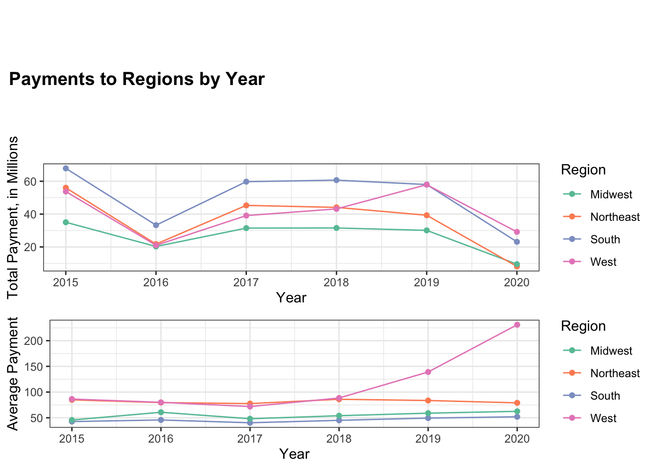
Again, for each year of the study, one-way ANOVA analysis was performed to determine if there was a statistically significant difference in payments to primary care physicians in different regions of the country. Each ANOVA returned a p-value of less than \(\alpha < 0.05\), so it seems there is a significant difference between the regions each year. Thus, with the figures above, it follows that physicians in the West and Northeast get statistically significant higher average payments than physicians in the South and Midwest.
| Years | P-value |
|---|---|
| 2015 | <0.001 * |
| 2016 | <0.001 * |
| 2017 | <0.001 * |
| 2018 | <0.001 * |
| 2019 | <0.001 * |
| 2020 | <0.001 * |
5.3 Temporal
5.3.1 Quarter of Year
Payments are now aggregated on a quarterly basis to determine if there is a difference in payment activity related to temporal trends. Over the study period, there does not seem to be a large difference in total payments to primary care physicians between the quarters for any given year. Likewise, there does not seem to be great differences in average payments. However, there does appear to be an outlier in average payments during Quarter 3 of 2020.
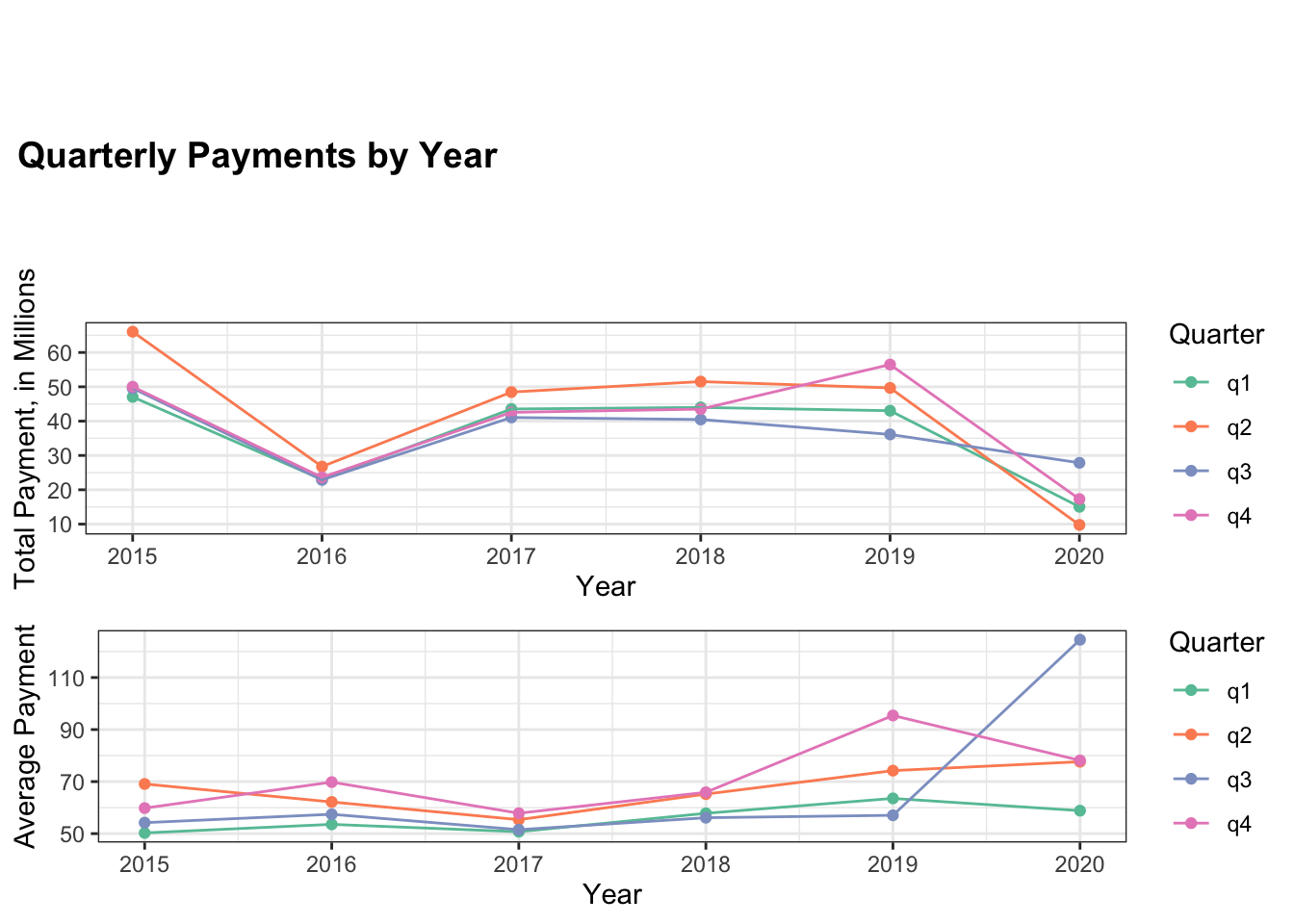
The one-way ANOVA analysis of differences in the quarters returned mixed results. While it found significant differences in 2015, 2017, and 2018, it did not return statistically significant results for 2016, 2019, or 2020. Thus, more temporal analysis is necessary.
| Years | P-value |
|---|---|
| 2015 | <0.001 * |
| 2016 | 0.061 |
| 2017 | 0.0291 * |
| 2018 | 0.0012 * |
| 2019 | 0.241 |
| 2020 | 0.213 |
5.4 Models
5.4.0.1 Linear Modeling
Now, this study considers how all the previous factors influence each other over each given year. The table below highlights the results of the linear model for 2019. The models for the other years can be found in the Appendix.
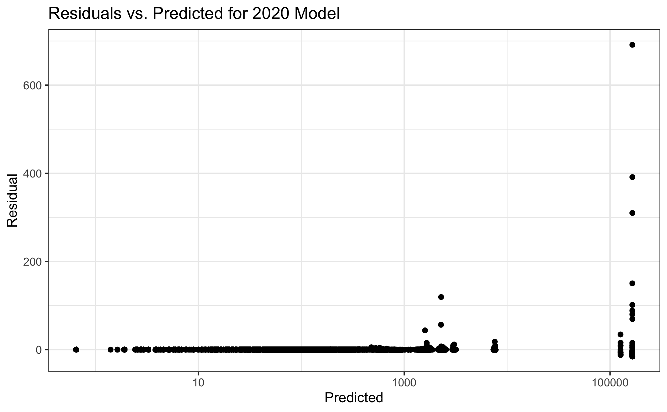
In fitting linear models, the residuals need to be examined. Here, there is extreme right skew, with the residuals being non-constantly variant. In fact, the residuals fan out as the predicted values increase. This trend holds for all models, i.e. there is right skew in the data for each year.
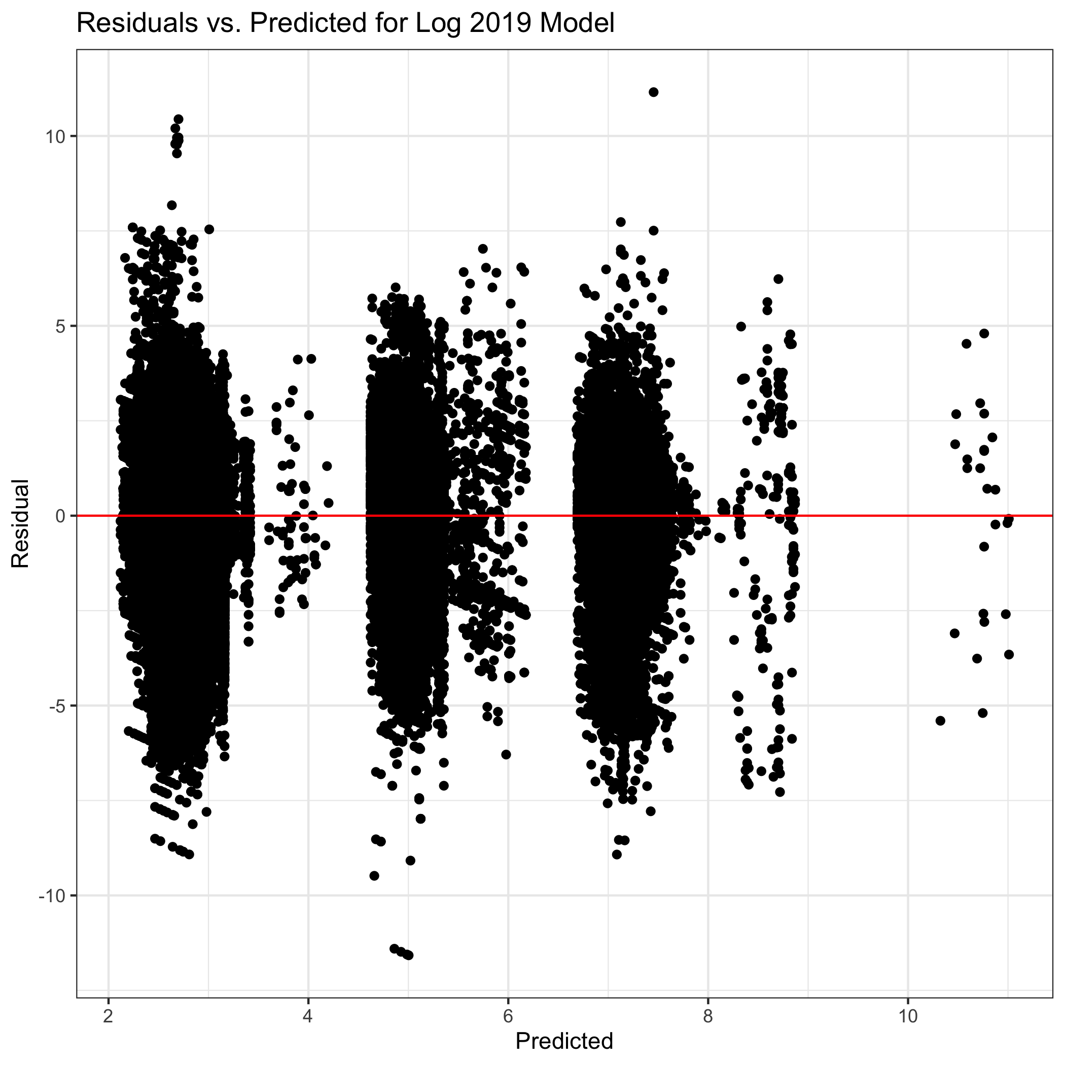
Thus, a log-transformation is applied to the dependent variable: payment value. Although there is right skew in the data, the residuals show that there is constant variance around a value of 0. Thus, the log-transformation of the total payments data is successful in achieving the linearity necessary for the linear model below.
The baseline for each model is the log payment to a primary care physician whose specialty is Family Medicine, has an extremely sparse ZIP code in the Northeast, and the payment is for “Compensation for services other than consulting” during the first quarter.
This model confirms many of the previous findings. There are significant differences between the regions and density categories, while there are mixed results for quarters of the year. Interestingly, it seems that a physician’s specialty may have predictive power, as there is a significant difference in log payments to Family Medicine physicians and physicians of all the other specialties. The nature of payment results also confirm what was found previously, showing that some payments have much higher values than others.
| Covariate | Coefficient | Std. Error | Statistic | P-Value |
|---|---|---|---|---|
| Intercept | 7.063 | 0.413 | 17.092 | <0.001 |
| Specialty: Family Medicine|Adolescent Medicine | 0.111 | 0.028 | 3.916 | <0.001 |
| Specialty: Family Medicine|Adult Medicine | 0.129 | 0.009 | 14.101 | <0.001 |
| Specialty: Family Medicine|Geriatric Medicine | 0.147 | 0.010 | 14.970 | <0.001 |
| Specialty: Family Medicine|Obesity Medicine | 0.266 | 0.044 | 6.122 | <0.001 |
| Specialty: General Practice | 0.319 | 0.002 | 129.471 | <0.001 |
| Specialty: Internal Medicine | 0.086 | 0.001 | 75.181 | <0.001 |
| Specialty: Internal Medicine|Adolescent Medicine | -0.134 | 0.015 | -8.965 | <0.001 |
| Specialty: Internal Medicine|Geriatric Medicine | 0.132 | 0.006 | 21.607 | <0.001 |
| Specialty: Internal Medicine|Obesity Medicine | 0.300 | 0.041 | 7.348 | <0.001 |
| Specialty: Pediatrics | 0.197 | 0.002 | 85.468 | <0.001 |
| Specialty: Pediatrics|Adolescent Medicine | 0.213 | 0.011 | 20.253 | <0.001 |
| Specialty: Preventive Medicine|Public Health & General Preventive Medicine | 0.574 | 0.021 | 26.803 | <0.001 |
| Nature of Payment: Compensation for services other than consulting | -0.084 | 0.413 | -0.204 | 0.838 |
| Nature of Payment: Compensation for serving as faculty or as a speaker for a non-accredited program | 0.151 | 0.417 | 0.361 | 0.718 |
| Nature of Payment: Compensation for serving as faculty or as a speaker for an accredited program | 0.484 | 0.433 | 1.116 | 0.265 |
| Nature of Payment: Consulting Fee | -0.264 | 0.413 | -0.639 | 0.523 |
| Nature of Payment: Current or prospective ownership or investment interest | 3.351 | 0.444 | 7.550 | <0.001 |
| Nature of Payment: Education | -4.807 | 0.413 | -11.632 | <0.001 |
| Nature of Payment: Entertainment | -3.366 | 0.425 | -7.918 | <0.001 |
| Nature of Payment: Food and Beverage | -4.528 | 0.413 | -10.957 | <0.001 |
| Nature of Payment: Gift | -1.513 | 0.414 | -3.654 | <0.001 |
| Nature of Payment: Grant | -0.381 | 0.415 | -0.919 | 0.358 |
| Nature of Payment: Honoraria | 0.097 | 0.414 | 0.235 | 0.814 |
| Nature of Payment: Royalty or License | 1.180 | 0.417 | 2.827 | 0.005 |
| Nature of Payment: Travel and Lodging | -2.334 | 0.413 | -5.647 | <0.001 |
| Region: South | -0.001 | 0.001 | -0.507 | 0.612 |
| Region: Midwest | -0.091 | 0.002 | -52.720 | <0.001 |
| Region: West | 0.030 | 0.002 | 17.031 | <0.001 |
| Density Category: Sparse | 0.037 | 0.002 | 22.456 | <0.001 |
| Density Category: Normal | 0.061 | 0.002 | 37.154 | <0.001 |
| Density Category: Dense | 0.111 | 0.002 | 66.452 | <0.001 |
| Density Category: Extremely Dense | 0.261 | 0.002 | 147.922 | <0.001 |
| Quarter 2 | 0.000 | 0.001 | -0.055 | 0.956 |
| Quarter 3 | -0.016 | 0.001 | -11.214 | <0.001 |
| Quarter 4 | 0.016 | 0.001 | 10.660 | <0.001 |
5.4.0.2 Time-series Modeling
Let us build a time-series model on average payments to primary care physicians for each quarter during the study period.
In applying the Holt-Winters method to average payments for each quarter, the model-predicted values appear to be somewhat similar to the actual values through 2019, but there is a large difference for the 2020 values.
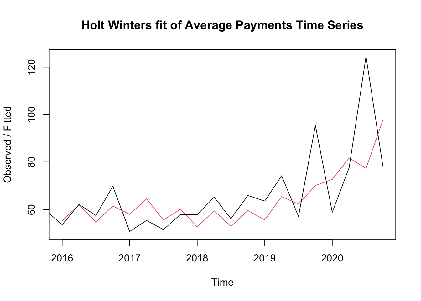
                   ME     RMSE      MAE       MPE     MAPE      MASE       ACF1
Training set 2.009594 13.41988 9.581064 0.3481101 13.43391 0.8763465 -0.4487789
For this model, the average difference between the fitted value and the actual value is MAPE = 13.43%. As highlighted above, the model seems to do particularly badly for the 2020 values. Thus, let us fit a new model for just the points from 2015 to 2019.
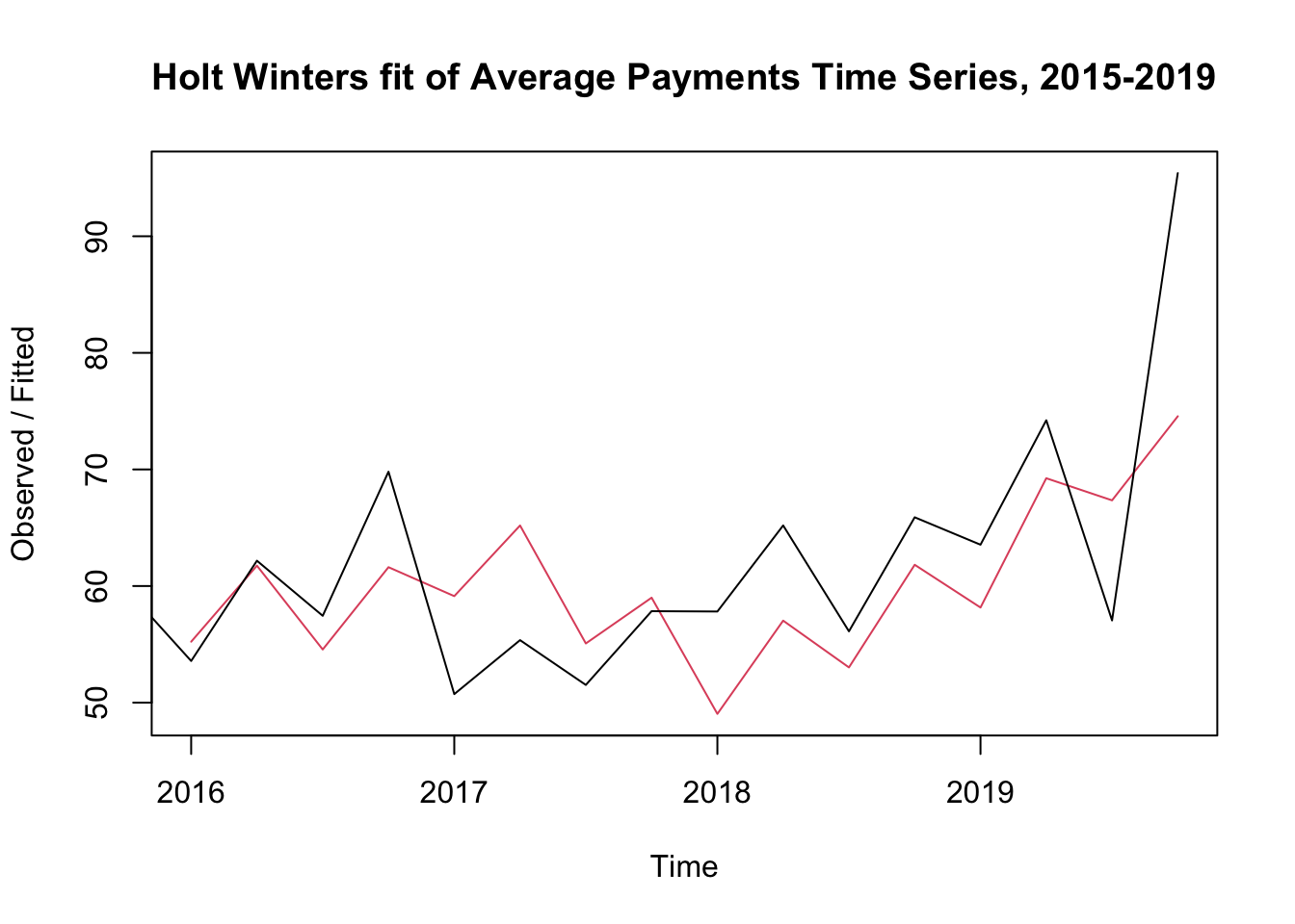
                   ME     RMSE      MAE      MPE     MAPE      MASE       ACF1
Training set 1.521215 9.433044 7.593289 0.594542 11.95973 0.9660007 -0.3993894
Without the 2020 data, the average difference between the fitted value and the actual value is MAPE = 11.96%. Thus, the 2020 data may introduce divergence from the trend present from 2015 to 2019.