Chapter 5 The Greeks
If there is one chapter you should master, it is without doubt this one.
Some examples in this chapter are coming from the excellent book of Peter Leoni: ‘The Greeks and Hedging Explained’. A must-read if you are interested by options.
5.1 Introduction to the Greeks
5.1.1 Introduction
Whenever a bank trades a derivative product, it ends up with a position that has various sources of risk. In practice, the bank does not risk manage each product independently. Instead, it adds each trade to its existing book of options and will risk manage this book globally. Indeed, some individual risks from different exotic products may offset each other.
Where do the various risks lie?
To answer this question, traders will need to know the sensitivity of their book to the market parameters.
These sensitivities are commonly referred to as the Greeks.
5.1.2 Taylor Series
To understand the concept of sensitivity we must first mention the Taylor series.
Any function can be approximated by a polynomial function. The coefficients for this polynomial are determined by the derivatives at a single point (understand the current market conditions in this case).
A first order approximation means that we are approximating the option price with a straight line. The second order approximation means we are using a parabolic shape.
Since option prices are convex with respect to some of their parameters, their linear approximations always lie below the exact option prices. The approximation generally gets better as we add more terms to it.
This simply gives us the various orders of sensitivities.
\(\boxed{\Delta V = \frac{\partial V}{\partial S} * \Delta S + \frac{\partial V}{\partial \sigma} * \Delta \sigma + \frac{\partial V}{\partial t} * \Delta t + \frac{\partial V}{\partial r} * \Delta r + \frac{1}{2} \frac{\partial ^2 V}{\partial S^2} * (\Delta S)^2 + Other}\)
The parabolic approximation is almost undistinguishable unless we move substantially from the initial level.
When pricing an exotic option, you will typically have to use some model. It is therefore fundamental that you understand well the model’s assumptions and their implications. Wrong models will typically result in wrong hedge ratios.
5.1.3 Static and Dynamic Hedge
A hedge is an investment made with the intention to offset or at least reduce the risk of a financial asset.
5.1.3.1 Static Hedge
A static hedge is a hedge that requires no changes to its components once it is initiated. In other words, the hedge won’t need to be re-balanced irrespective of how the market moves.
If a financial product has all its cashflows aligned with those of liquidly traded instruments, then a static hedge can be put into place and this static hedge is model independent. The price of the financial product is then nothing but the cost of setting up the static hedge.
The existence of a static hedge therefore provides us with both a price and a hedge!
Unfortunately, for most of the exotic products covered in this material, such a static hedge is not possible and a dynamic hedge must be implemented.
5.1.3.2 Dynamic Hedge
Unlike a static hedge, once a dynamic hedge is initiated, it is sensitive to movements in the market and must be readjusted to still be a hedge.
The frequency at which the hedge must be rebalanced depends on the nature of its sensitivities and its impact on the price.
The initial hedge is generally made up two parts:
- A static part that does not require any further adjustment.
- A dynamic part that will need to be adjusted through the product life.
5.1.4 Summary Table of the Greeks
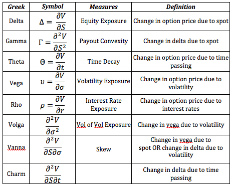
Fig: 5.1 : Summary Table of the Greeks
We will see why these greeks are relevant and how they do their job. We will see their features and behaviours when new market conditions develop.
Note that all the conclusions can easily be drawn by understanding the time value of an option. This by itself will turn out to be enough to qualitatively understand the behaviour of the Greeks! The quantitative understanding requires the expressions provided by the model.
5.2 Delta
5.2.1 Description
Delta is the first-order sensitivity of the price to a movement in the spot price, S. It gives the equity sensitivity of the option and is closely related to the probability of the option finishing in-the-money (but different…).
Delta is normally quoted in percent and gives how much of percentage of the actual stock is required to hedge the option.
5.2.2 Calls
For calls, delta lies between 0% and 100%:
- Far OTM calls have delta near 0% meaning there is little to no equity sensitivity.
- Far ITM calls have delta close to 100% meaning that they trade like a stock.
- ATM calls have delta around 50%.
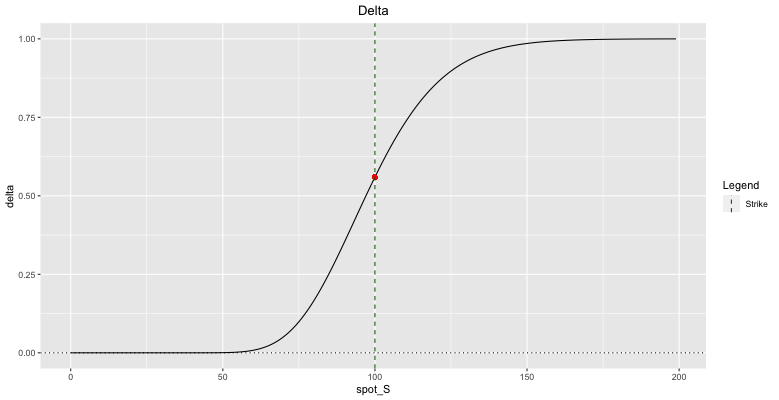
Fig: 5.2 : Call Delta
5.2.3 Puts
For puts, delta lies between 0% and -100%:
- Far OTM puts have delta near 0% meaning there is no equity sensitivity.
- Far ITM puts have delta close to -100% meaning that they trade like a short stock position.
- ATM puts have delta around -50%.
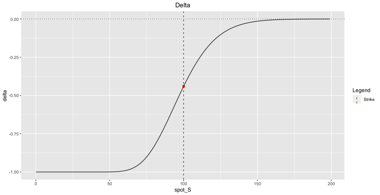
Fig: 5.3 : Put Delta
As you can see, the delta for calls and puts have the same shape. This is a direct consequence of the call-put parity!
Both deltas are increasing with the stock value.
If there is a small movement in the spot price S, then the price of the derivative will move by delta times this small movement. For example, a delta of 0.5635 means that if the underlying asset moves by 1, then the value of the derivative will move by 0.5635 × 1.
Note that the delta of a book of options is the sum of the individual deltas.
5.2.4 Assets to delta hedge
To delta hedge, one can use the underlying asset itself, forwards or futures on the underlying asset or another correlated asset.
5.2.4.1 Delta Hedging using Forwards/Futures
Assuming no dividends, the forward price at time t with maturity T is given by \(F_t= S_t \; e^{r(T-t)}\) so that the delta of the futures contract is given by \(e^{r(T-t)}\). To match a particular delta of \(Δ_S\) with a position in a futures contract on the underlying, you will require a position of \(e^{-r(T-t)} \; Δ_S\) in the futures contract.
5.2.5 Delta under Black-Scholes
Under Black-Scholes assumptions, deltas for call and put options on non-dividend paying stocks are given by:
\(\boxed{\text{Call Delta} = \frac{\partial C}{\partial S} = N(d_1)}\) and \(\boxed{\text{Put Delta} = \frac{\partial P}{\partial S} = N(d_1) - 1}\)
where:
- \(N()\) is the standard Normal Cumulative Distribution Function
- \(d_1 = \frac{\text{ln} \left( \frac{S}{K} \right) + \left( r \; + \frac{\sigma ^2}{2} \right) t}{\sigma \sqrt t}\)
The delta of a European option is therefore sensitive to:
- the time to expiry (t).
- the volatility of the underlying (\(\sigma\)).
- the moneyness (\(\frac{S}{K}\)).
On a dividend-paying stock, the BS deltas are simply multiplied by \(e^{-qt}\), where q is the dividend yield.
5.2.6 Delta sensitivities
5.2.6.1 Impact of Time to Maturity
At maturity, delta has a digital shape around the strike. Once we move ourselves away from maturity, the delta becomes much smoother shaped. The further we are from maturity, the flatter the curve looks.
The delta converges faster and faster to its intrinsic value as time to maturity goes to zero. The option picks its direction. That is true, except for ATM option, where the delta remains flatter.
Main variation from the delta is always located in the ATM range. The closer we are to maturity, the tighter the range is where the delta changes from small value to full value.
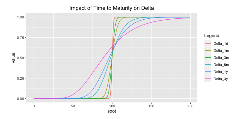
Fig: 5.4 : Impact of Time to Maturity on Delta
Since delta hedging is uncertain and implies transaction costs, there is a willingness to keep it to a minimum. In practice, delta hedges are usually done on a daily basis.
Since time impacts delta, one should adjust its effect on delta for weekends and holidays even though the underlying does not move during these days! The closer to maturity, the more important this adjustment.
The effect of time on delta is represented by a second-order sensitivity called the charm.
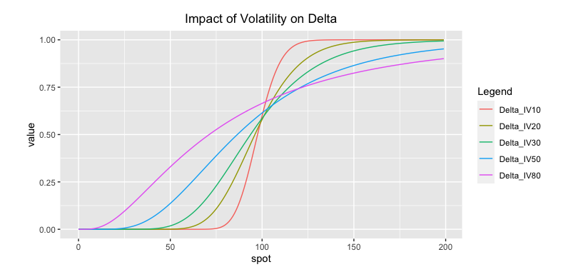
5.2.6.2 Impact of Volatility
The trader wants to know and understand how the delta will change when volatility changes. It will allow him to anticipate the hedge adjustments and take a position accordingly.
A higher volatility increases the delta for OTM options. The more volatility, the less OTM an OTM option really is.
A higher volatility decreases the delta for ITM options. The more volatility, the less ITM an ITM option really is.
More volatile stocks therefore have a less pronounced delta.

5.2.7 Other factors linked to delta hedge
5.2.7.1 Liquidity
Liquidity is also a concern. A trader will adjust his price if the underlying stock is illiquid and difficult to trade. For example, if a stock is hard to short, then borrowing costs will have to be factored into the price.
5.2.7.2 Dividends
As sellers of structured products, banks are structurally long the underlying assets as their delta hedge consists of buying delta on these assets. Being long underlying means they are also long dividends. To obtain a correct option price and hedge, dividends will have to be taken into account.
However, dividends are uncertain. So, how should dividends be factored into the price?
It can be done in two ways:
- either in the form of a term structure of dividend yields.
- either priced at current levels and hedged using dividend swaps.
On a book level, exposures to dividends can be significant and will need to be hedged.
5.2.7.3 Interest Rates
To buy delta, a trader has to borrow money. If interest rates go up, borrowing becomes more expensive making the hedging process and therefore the option price more expensive. The sensitivity of an option price to interest rate movements will be further discussed in the section on Theta.
5.2.8 Delta as a hedge ratio, not a probability
We said that delta was closely related to the probability of finishing ITM and used it sometimes this way as it is quite intuitive for option rookies. I must emphasize again that they are not the same thing. This can be intuitively shown with a small extreme binary example.
A stock is trading for 10€ and tomorrow there is a ruling:
- 10% of the time the stock goes to 100.
- 90% of the time the stock goes to 0.
As you can see, it is correctly priced as 10€ represents the expected value.
What would be the price of an OTM call with a strike @ 50€?
As usual, the price will be the discounted expected value of the cashflows. Discounting does not matter here as it is on a very small time step (1d) so the expected value is 0.1*50€ = 5€. The call is worth 5€.
What would be the delta of this OTM call?
Delta = \(\frac{\Delta C}{\Delta S}\)
In the down case, the call goes from 5€ to zero as the stock goes from 10€ to zero. Delta = \(\frac{5€}{10€} = 0.5\).
In the up case, the call goes from 5€ to 50€ while the stock goes from 10€ to 100€. Delta = \(\frac{45€}{90€} = 0.5\).
The call has a 0.5 delta.
In this binary example, the 400% OTM call has a 50% delta despite only having a 10% chance of finishing ITM.
We used this binary example to show that delta is different from the probability of finishing ITM. If you take a more balanced distribution, the two will be closer to each other though.
You could summarize things as follows: the more positively skewed the distribution, the more the delta diverges from the probability of finishing ITM (the further OTM the 50% delta call will be).
In this regard, you can also think of the impact of volatility on delta based on its impact on the distribution. The higher the volatility, the more positively skewed the distribution, the further OTM the 50% delta call will be.
If you are skeptical about the impact of volatility on the distribution, more volatility increases the upside of possible payoffs but decreases the probability of the stock going up and increases the probability of the stock going down.
In case you were wondering, this intuition is perfectly in line with the Black-Scholes framework previously described.
In BS, the call delta is N(d1) while its probability of finishing ITM is N(d2). Remember the relationship between d2 and d1 is: \(d2 = d1 - \sigma \sqrt{t}\)
So the higher the volatility, the more delta and probability of finishing ITM will diverge.
I hope this discussion will allow you to avoid the common misconception that ATMF (at-the-money-forward) call and put have the same delta. They have the same price by the call-put parity!
5.2.9 Setting up a small delta-hedging experiment
Let us try to understand how to manage a book of derivatives. Suppose we know the stock is following the Black-Scholes dynamics. We could then analyse how the delta hedge procedure works. If this theory is solid, we should be able to eliminate all risks while hedging.
5.2.9.1 Market conditions
- Interest rates are at a 2% level –> r = 0.02.
- Underlying stock pays no dividend and follows a Geometric Brownian Motion (GBM) with µ = 10% and σ = 20%.
- The initial spot price is \(100€\) –> \(S_0 = 100\)
- The call option is ATM with a maturity of 0.1 year –> T = 0.1
We are going to delta hedge at regular time step with dt = 0.005 so that there are 20 steps. We will generate sample paths of the stocks by generating standard normal deviates and use the known formula. From the time series, we can calculate back the realised volatility after the experiment –> realized volatility = 17%.
5.2.9.2 First Day
The trader sells the option at a price of 2.62€, corresponding to an implied volatility of 20%. He will also use this implied volatility for hedging purpose, which prescribed a delta of 52.52% so that he buys 0.5252 stocks. He does this by borrowing \((0.5252*100€ - 2.62€) = 49.90€\).
After the first day, the trader has the following instruments in his book:
- A sold call option at \(2.62€\).
- A loan with a present value of \(49.90€\).
- A stock portfolio with a value of \(52.52€\).
5.2.9.3 Second Day
The outstanding loan is increased because of the interest effect. In this case, the effect is about 1 cent. The stock has decreased by 10 cents. Because of the delta-position, his stock portfolio loses about 5 cents. The sold option loses more than just 5 cents.
All of this brings the trader’s book at a positive value.
After the change in the market, the delta has changed to 41.83%. The trader will thus sell part of his stock portfolio at the current level. With this cash, he pays back part of the loan. The trader is in a new delta-neutral position to start the next day.
5.2.9.4 Observations
The theory of Black-Scholes is prescribing that the hedging cost leads to the option price. However, we notice a profit coming into the book after just one day of hedging! Why?
The reason is that the theory assumes that you are hedging continuously through time, rather than once a day. So the error is induced by the discrete nature of the hedging strategy.
Another way of looking at this is by analyzing the random number that was used to generate the value of the second day. This number is a draw from the standard normal distribution. This one is a small number.
One could say that the volatility of the first day, because of this small draw, is smaller than actually predicted by the distribution. It is smaller than the “typical” number in a standard normal distribution.
Which random number one has to use in order to see no profit and no loss in this first day?
Z = -1 or +1 –> one standard deviation out of the mean.
5.2.9.5 Conclusion
Every day where the move of the stock is less than anticipated, based on volatility, the trader will have a gain in his book.
Every day where the move of the stock is bigger than anticipated, based on volatility, the trader will have a loss in his book.
Because of the statistical nature and the assumed independence of the moves on a daily basis, his losses and gains will average each other out, at least if the volatility that realizes corresponds to the pricing volatility at the start.
What happens if right after the price agreement has been done, the market volatility drops to 5%?
This means that the trader will see a nice profit in his book. However, this profit will die out if trader hedges the option during the lifetime, because the final P&L will depend on how the realized volatility turns out. The smart trader would try to buy back this option in the market if possible and hence lock in this margin.
As we explained in this delta-hedging procedure, there are discrete effects. Up to now, we only have a qualitative understanding of those. No worries, the introduction of gamma and theta will help us quantify them.
5.3 Gamma
5.3.1 Description
Gamma measures the change in delta due to the change in underlying price. It represents the second-order sensitivity of the option to a movement in the underlying asset’s price. The higher the gamma, the more convex the theoretical payout.
Be careful that gamma is not a measure of value! A low/high gamma option does not mean a cheap/expensive option. An option’s implied volatility is a measure of its value, not its gamma.
The price of an option as a function of the underlying price is non-linear. Gamma allows for a second-order correction to delta to account for this convexity.
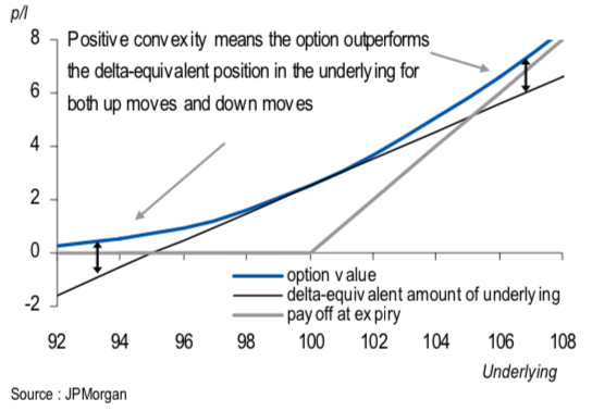
Fig: 5.6 : Option Convexity
This convexity in the underlying price is what gives the option value. It is important as it enables the traders to derive the profit on an option for any given stock move.
A delta-hedged portfolio is a portfolio that has been hedged by trading in the underlying asset against small movements in these assets (black line).
As a second-order effect, the gamma becomes significant when large move in the underlying occurs (convexity seen in the blue curve).
As we can see in the above figure, a long position in option is convex and there has a positive gamma. To delta hedge, the trader will need to sell stocks if the stock price goes up and buy stocks if the stock price goes down (sell high – buy low). The trader can sit on the bid and offer.
A short position in option is negative gamma. In this case, the trader will need to sell stocks if the stock price goes down and buy stocks if the stock price goes up to be delta hedged (sell low – buy high). The trader has to cross the bid-offer spread.
5.3.1.1 Gamma Hedging
To hedge this gamma, we need to trade other convex instruments such as other European options so that gammas cancel out. A lower gamma means that we will have a lower need for large and frequent rebalancing of delta.
To see the second-order effect in pricing, we will use models that assume some form of randomness in asset’s price.
5.3.2 Gamma under Black-Scholes
Gamma for both calls and puts are the same.
This is not surprising at all. We have seen that gamma was the first derivative of delta with respect to the underlying price and that the graphics of delta for calls and puts were similar.
This can easily be seen mathematically. Since the delta of a call for a non-dividend-paying stock is given by \(Δ_C=N(d_1)\) and the delta of a put on a non-dividend-paying stock is given by \(Δ_P=N(d_1)-1\), differentiating with respect to the spot price has the same effect!
\(\boxed{\text{Put Gamma} = \text{Call Gamma} = \Gamma = \frac{\partial ^2 C}{\partial S^2} = \frac{\partial \left( \frac{\partial C}{\partial S} \right)}{\partial S} = \frac{\partial N(d_1)}{\partial S} = \frac{\partial N(d_1)}{\partial d_1} \frac{\partial d_1}{\partial S} = N'(d_1) \frac{\frac{1}{S}}{\sigma \sqrt t} = \frac{N'(d_1)}{S \sigma \sqrt t}}\)
Since deltas of both calls and puts are increasing with the stock value, gamma is always positive for a long option position.
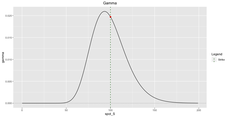
Fig: 5.7 : Option Gamma
When learning about delta, we have seen that most of the change in the delta occurs around the ATM point. So the gamma should be large around this point! As the spot price moves away from the strike, \(N'(d_1)\) will become small and gamma will rapidly decrease. This can be observed in the above figure where the gamma of a call option is plotted. Notice how it resembles the bell-shaped curve of the Normal distribution.
As we move into exotic structures, we will see that these may have quite different Gamma profiles to the European options. Their gamma can change sign!
Note that the gamma of a portfolio of options is also the sum individual gammas of the options.

5.3.3 Gamma sensitivities
5.3.3.1 Moneyness
Gamma tells us how much delta will move if the underlying moves. Gamma generally has its peak value close to ATM and decreases as the option goes deeper ITM or OTM. Options that are deeply ITM/OTM have gamma close to zero. This behavior is obvious when looking at figure 5.7.
5.3.3.2 Time to Maturity
We have seen that delta get smoother for larger time to maturity. So we can expect a smoother gamma for a longer maturity.
As the time to expiration draws nearer, gamma of ATM options increases while gamma of ITM/OTM options decreases.
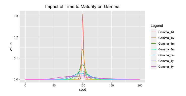
Fig: 5.8 : Impact of Time to Maturity on Gamma
5.3.3.3 Volatility
We have seen that volatility attacked the delta, so it is not surprising it weakened the gamma too. Since a higher volatility induces a less pronounced S-shape delta curve, it also induces a less pronounced/wider more stable bell-curved gamma.
A higher volatility lowers the gamma in the ATM region and increases the gamma in the ITM/OTM regions.
It is very easy to think about this effect in terms of time value of options.
For low levels of volatility, deep ITM/OTM options have little time value and can only gain time value if the underlying asset moves closer to strike.
For high levels of volatility, both ITM/OTM options have time value and the gamma near strike should not be too different from away from strike. Therefore, for high levels of volatility, gammas tend to be more stable across all strike prices.
We can say that volatility weakens the gamma.
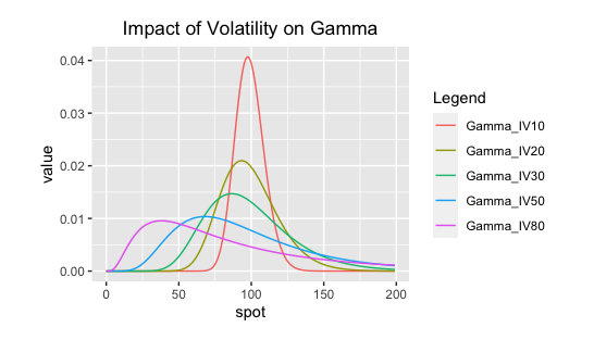
Fig: 5.9 : Impact of Volatility on Gamma
5.3.4 Negative Gamma at maturity is tricky
The gamma of a European option is high when the underlying trades near the strike and there is little time left to maturity. Around this point, the trader will need to delta hedge more frequently, making the hedging process more expensive.
Intuitively, the delta of a call option on the day of expiry will change from roughly 0% when the spot is lower than the strike to roughly 100% when the spot is larger than the strike.
Therefore a small change in spot will result in a large change in delta and gamma is very high.
Any trader that has sold options can tell you how tricky it is to manage the book near maturity when the spot is around the option’s strike. The gamma gets so big that the hedging needs to be done very fast. As he is the option seller, he is gamma short, with a huge gamma position. If the market keeps moving around the strike, every rebalance will cost him money and the amount of theta for is limited.
In some cases, in highly volatile markets, it is sometimes better to either fully hedge at once or fully unwind. If you are wrong, it will cost you, but rebalancing can be even more costly (slippage or bid/offer spreads).
5.3.5 Gamma P&L
This section is taken from the article on variance swaps written by the Equity Derivatives Research from JP Morgan. I will heavily rely on this excellent article when writing about variance swaps.
Options are exposed to a wide range of factors such as: performance of the underlying asset, time, volatility, interest rates, dividends, etc.
The first-order exposure to moves in the underlying can be hedged out by the familiar delta-hedging process. This leaves the exposure to volatility, paid for in time-decay as the most important sensitivity. However, this is not a pure volatility exposure as it is path dependent!
Suppose we hold a call option. To be delta-neutral, we can sell an amount of the underlying equivalent to the delta of the option. By frequently re-adjusting this delta-hedge, sensitivity to asset moves can be dynamically hedged out over option’s lifetime.
P&L will come from the accumulated action of continuously re-balancing to keep the portfolio delta-neutral over time. The gamma P&L is paid for in the option premium, which is marked to market as lost theta.
How is this gamma P&L actually made ?
Essentially the gamma measures the convexity of the option. This convexity always works in favour of long options positions.
For small moves in the underlying, the replicating hedge is accurate. For larger moves in the underlying, the long options position is always outperforming the replicating hedge in both directions. This is the principle of the convexity by itself. The first derivative of a convex curve is always below the curve itself.
For a delta-hedged option, the gamma P&L will be the outperformance of the option over the replicating hedge. The more the delta changes, the more the replicating delta-hedge will underperform the long options position.
How much will it underperform?
The actual amount depends on the difference between the initial and final delta of the option, which is gamma time the change in the spot price.
Let us assume that gamma remains constant and see how the gamma P&L can be calculated.

Fig: 5.10 : Gamma P&L from delta-hedged options
- Initially, the underlying spot price is \(S_0\), the option is worth \(p_0\), delta and gamma are respectively \(Δ_0\) and \(Γ_0\).
- The spot then increases by dS to \(S_1\).
- The delta increases to \(Δ_1= Δ_0+ Γ_0 \; dS\).
- The average delta is therefore: \(Δ_{avg}= Δ_0+ \frac{Γ_0 \; dS}{2}\).
- The new option premium is worth \(p_1= p_0+ Δ_{avg} \; dS\).
- Replacing \(Δ_{avg}\) with 3., we have: \(p_1 = p_0 + Δ_0 \; dS + \frac{Γ_0 \; dS^2}{2}\).
- The P&L on the long option position is: P&L = \(p_1 - p_0 = Δ_0 \; dS + \frac{Γ_0 \; dS^2}{2}\).
- The P&L on the short delta-hedged position is: P&L = \(-Δ_0 \; dS\)
- The total P&L is therefore: Total P&L = 6. + 7. = \(\frac{Γ_0 \; dS^2}{2}\).
So the gamma P&L, which is the difference between the performance of the option and the replicating delta hedge is \(\boldsymbol{\frac{1}{2} * \Gamma * dS^2}\).
The gamma P&L from a move in the underlying is proportional to:
- the gamma of the option, (\(Γ\)).
- the square of the move, (\(dS^2\)) –> gamma P&L from a 2% move will be four times that of a 1% move!
5.3.6 An example
A trader is long gamma through buying a put option. If the market is right and balanced, the trader paid a fair price so that the money he can expect to make will be paid for through premium.
Assume the market suddenly realizes that the option was underpriced. Expectation now becomes that the stock will be more volatile so that the implied volatility increase and the option becomes more expensive in the market.
The trader has a choice. He can keep on delta hedging and profit from this highly volatile market or he can cash in and sell the option at a higher price.
How much money can he expect to make over the lifetime of the option if he continues hedging himself?
That amount can be shown to be identical to cashing in right now. Underlying this statement, there is the assumption that the implied volatility turns out to be the correct one.
This actually gives the trader an interesting dilemma. Because the market will keep changing his mind over time about the best implied volatility that has to be used. Option traders will take positions when they think the implied volatility is low/high. The money they will pick up by trading is directly related to the vega of these options.
5.3.7 Can volatility be captured by delta-hedging?
We have seen how the gamma P&L was made by benefiting of the volatility when delta-hedging. This exposure to volatility is not a pure volatility exposure as it is path dependent!
Suppose a market maker buys and delta-hedges a vanilla option. Assuming that whatever volatility is realized is constant and option is delta-hedged over infinitesimally small time step, then the market maker will profit if and only if the realized volatility is larger than the implied volatility at which the option was purchased.
However, volatility is not constant! Where and when the volatility is realized is crucial! Furthermore the magnitude of the P&L depends not only on the difference between realized volatility and implied volatility, but where that volatility is realized in relation to the option strike.
If the volatility realizes close to maturity when the underlying trades near the strike then the gamma would be very high and the absolute value of the P&L will be larger.
For non-constant volatility, it is possible to buy and delta-hedge an option at an implied volatility smaller than the subsequent realized volatility and still losing money from delta-hedging!
5.3.7.1 Example with a 1-year SX5E option
The SX5E index is initially quoting at 3500 with an ATM implied volatility of 28.5%. During the first seven months, the index ranged between 3500 and 3800 points, realizing a volatility of 20%. After that period, the index fell rapidly to 2500 points, realizing approximately 50% volatility on the way. Over the whole year, the realized volatility was 36%.
Case 1: Long 2500-strike option @ 33.4%
Suppose a trader is long a 2500-strike option at an implied volatility of 33.4% due to the skew observed in the market.
Initially, the option made a loss due to low realized volatility. However, the loss was kept small thanks to the low gamma exposure as the spot was trading far from the option strike.
As the SX5E sold off, the option gamma increased while volatility picked up and the option ended up making a large profit!
Case 2: Long 4000-strike option @ 26%
Suppose a trader is long a 4000-strike option at an implied volatility of 26% due to the skew observed in the market.
Initially, the option has a higher gamma and lost more due to lower realized volatility.
As the index sold off and volatility occurred, delta-hedging failed to capitalise on it because the gamma was very low far from the strike.
Despite the fact that the option was purchased at an implied volatility 10% below the subsequent realized volatility, it ended up losing money!
\(\underline{\text{Conclusion}}\)
When delta-hedging daily an option, the P&L is a daily accrual that depends on the difference between the realized volatility and the implied volatility. The magnitude of the contribution of this daily accrual is weighted by the current dollar gamma, which is unpredictable since path-dependent!
5.3.8 Dollar Gamma
Remember the formula of gamma given previously: \(\boxed{\Gamma = \frac{N'(d_1)}{S \sigma \sqrt t}}\)
Since \(N'(d_1)\) is independent of the monetary units of the underlying, gamma will be inversely proportional to the value of the underlying (S at the denominator of the formula).
Gamma is a very useful concept but it has two drawbacks:
- It measures the change in delta per unit of underlying.
- It is dependent on the absolute level of the underlying.
Moving to the concept of the dollar-gamma is more useful because:
- It allows us to directly calculate the gamma P&L for a given percentage underlying move.
- It makes it much easier to compare gamma exposures across different underlyings.
Dollar delta is the cash equivalent exposure of the underlying.
Dollar gamma is the change in the dollar delta for a 1% move in the underlying.
It can easily be shown that \(\boxed{\boldsymbol{\$\Gamma = \frac{\Gamma \; S^2}{100}}}\)
If S changes from S to \(S + \frac{S}{100}\), then \(Δ\) changes from \(Δ\) to \(Δ + \frac{ΓS}{100}\) and \(\$Δ\) changes from \(\$Δ\) to \(\$Δ + \frac{ΓS^2}{100}\).
For a return R, it can also be shown that \(\boxed{\boldsymbol{gamma \; P\&L = 50 \; \$\Gamma \; R^2}}\).
Remember that if S changes to S + dS, then the gamma P&L would be \(\frac{\Gamma \; dS^2}{2}\).
We have just seen that \(\$\Gamma = \frac{\Gamma \; S^2}{100}\). By isolating \(\Gamma\), it can be rewritten as: \(\Gamma = \frac{100 \; \$\Gamma}{S^2}\).
Replacing this expression into the previous one, the gamma P&L can be written as: \(\boxed{\frac{100 \; \$\Gamma}{S^2} * \frac{dS^2}{2} = 50 \; \$\Gamma \; (\frac{dS}{S})^2 = 50 \; \$\Gamma \; R^2}\)
For example, if we hold a position which is long \(\$100.000\) of dollar gamma and the underlying asset moves by 3%, then the P&L will be \(50*\$100.000*(0.03)^2 = \$4.500\).

5.4 Theta
5.4.1 Description
There is no free lunch in the world of finance. The story would be too good to be true if holding a call/put and dynamically rebalancing gave a profit due to gamma.
Positive gamma does not come for free.
We will now explain where the paradox is coming from. We left out one very important feature. The trader who owned the option and was making free gamma money out of it had to pay the premium in the first place. The profit he makes afterwards has to make up for this premium payment.
An option holder pays for the right of buying low and selling high by means of the theta, the time decay of an option. The holder of an option needs to earn back the daily loss of the option by taking advantage of the underlying’s moves.
The seller of an option makes money on the theta and loses it by rebalancing delta by buying high and selling low.
The longer the lifetime of the option, the more time to move further ITM, the more expensive the option should be. So we know that the value of the option becomes worth less and less with every day that passes by. This process is inevitable. So little by little the option loses its value.
The change in value from one day to the next is called the theta. Clearly this number is expected to be negative for both ATM call and ATM put option.
5.4.2 Theta under Black-Scholes
Theta is defined as the rate of change of the option price respected to the passage of time: $ $.
Instead of measuring the passage of time all else being equal, we also could simply investigate the same option with an expiry of one day earlier. Both approaches are identical within Black-Scholes as the Brownian Motion is a stationary process. In terms of formulas, we can therefore write: \(\boxed{\Theta = \frac{\partial V}{\partial t} = \frac{\partial V}{\partial T} \frac{\partial T}{\partial t} = \frac{\partial V}{\partial T} (-1) = \; - \frac{\partial V}{\partial T}}\)
Under Black-Scholes assumptions, thetas for call and put options on non-dividend paying stocks are given by:
\(\boxed{\text{Put Theta (per year) = } \Theta = \; - \frac{S \sigma}{2 \sqrt T} N'(d_1) + rK e^{-rT} N(-d_2)}\)
\(\boxed{\text{Call Theta (per year)} = \Theta = \; - \frac{S \sigma}{2 \sqrt T} N'(d_1) - rK e^{-rT} N(d_2)}\)
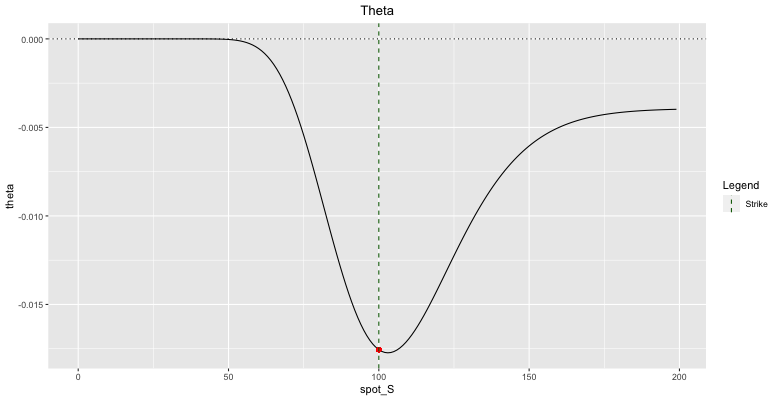
Fig: 5.11 : Call Theta
5.4.3 Some features of Theta
Let us turn to an example that will unfold the finesse of the Greek that makes you lose. Let us assume that the underlying stock does not pay any dividend and has a spot price of 20, interest rates are at 2.5%. A 1-year ATM put is quoting 2.5€ for an implied volatility of 35%.
Suppose there are 250 trading days in a year as we assume the option only loses value on working days.
We could write a fixed loss of \(0.01€/day\) in our book. It would make the loss of time value completely predictable. However, there would be an inconsistency between the market value and the booked value!
By accepting a marked-to-market valuation, we have to accept that:
- We only know the theta today.
- We also know all time value will have disappeared when we reach maturity.
- But we cannot predict how the time value will behave over time!
In fact, the theta exhibits several features:
- theta loss speeds up as maturity approaches.
- theta depends on moneyness.
- theta is strengthened by volatility.
5.4.3.1 Theta Speed of loss
The option loses little value at the start and this process speeds up as maturity approaches.
5.4.3.2 Theta depends on moneyness
The real potential of an option is found in the ATM range.
Let us take an example where we buy an ATM put initially and imagine different scenario.
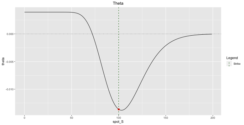
Fig: 5.12 : Put Theta
Note that at first sight the theta is negative, there are 2 situations where it turns positive.
Far ITM put options are known to have positive time decay (see figure 4.12). Remember we have seen that the time value of ITM put options can be negative, so nothing really surprising here!
For ITM call options, the theta can turn positive as well, in the case where the dividend yield is larger than interest rates so that the forward level is below the current spot level. Figure 4.11 does not reflect this as it plots the Theta of a 1-year call option on a non-dividend-paying stock in a positive interest rate world.
Case 1 : From ATM to ITM
Initially the put option is ATM but then the stock moves down and the put price rises.
Although the put value increased, the time value is less than for ATM option. Clearly, if the time value is less altogether, there is less value to lose when time passes.
Case 2 : From ATM to ITM then back to ATM
Suppose the trader owns an ATM put option.
During the first week, the stock does not move so that both time value and option value decrease.
During the second week, the stock drops by 10% so that option price increases (due to intrinsic value) and time value decreases.
We know that if the time value is smaller, the daily decrease in time value is lower than before the actual move.
If the stock moves back up to the ATM level, the option value goes down but the time value increases. As of then, the daily decrease in time value is more substantial than before this move back up.
How all the changes in time value add up ?
This is the topic of the next section, where we see the theta in relation to the gamma.
Over the lifetime the sum of all changes in time value on a daily basis just add up to the option premium of the first day.
The reason behind this is nothing else but the fact that an option converges to its intrinsic value.
The creation of extra time value is a temporary effect.
5.4.3.3 Theta is strengthened by Volatility
The higher the volatility, the higher the option price and the time value, the more time value to lose, the larger the absolute value of theta.
As the vega is higher in ATM region, the effect is larger in this region so that the theta change is most noticeable when ATM. The higher the volatility, the wider this ATM region.
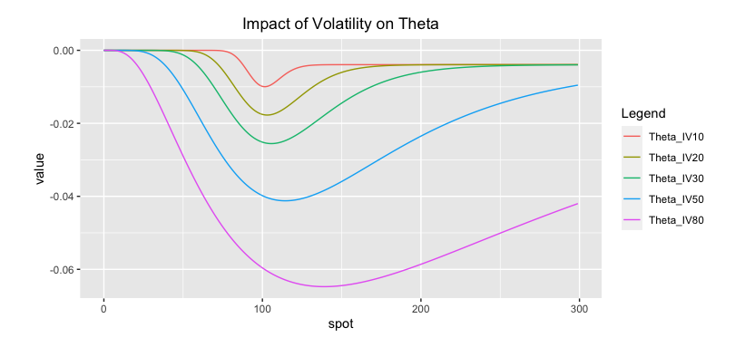
Fig: 5.13 : Impact of Volatility on Theta
5.4.4 Gamma and Theta are always flirting
There is no free lunch in owning an option.
You will make free gamma money and you will lose precious theta money. There is a balance to be found.
A trader that bought an option paid the intrinsic value (if any) and the time value. He knows the time value will be lost during the lifetime of the option. The only thing he does not know is how big the future daily losses/gains will be. However, the sum of all these will have to make up for the extrinsic premium paid. He will have to work for his money by actively delta hedging and locking in the gamma profits.
Every single day the trader who owns the option tries to fight the theta by:
- rebalancing his portfolio at appropriate times.
- leaving the position open if he expects the stock to keep on moving in the same direction.
By waiting, he gets to lock even more profit in one single rebalance but he is taking a risk.
5.4.4.1 Derivation of Black-Scholes equation
Within the Black-Scholes setup, we can derive an expression that exactly specifies this relation between these two greeks:
\(\boxed{\Theta + \frac{1}{2} \Gamma S^2 \sigma^2 = r(V - \Delta S)}\)
This relation is interesting because it is telling us how all the different Greeks lead to the price. We know that the cost of any derivative is determined by the cost of hedging.
Let’s first consider a portfolio of an option that we will delta hedge.
On the cash part, we have the option premium V and the loan with value equals to the value of the stock holdings in the portfolio, \(∆S\).
The interest accumulated over short time interval \(∆t\) on this net amount is: \(\boxed{r(V - \Delta S) \; \Delta t}\)
That is the deterministic cost of the construction.
On the dynamic hedging procedure, we know we will lose the amount of theta, \(Θ\).
The \(Γ\) term requires slightly more attention to explain. The \(Γ\) profit would be given by: \(\boxed{\frac{\Gamma \; (\Delta S)^2}{2}}\).
Since the volatility is relative, we need to multiply it with the current level of the stock to get an absolute number.
In a time interval ∆t, the typical movement would be: \(\boxed{\Delta S = S \sigma \sqrt{\Delta t}}\).
So the combination of theta and gamma effect over ∆t is given by: \(\boxed{\Theta \Delta t + \frac{1}{2} \Gamma S^2 \sigma^2 \Delta t}\)
Taking all together, we have: \(\boxed{\Theta \Delta t + \frac{1}{2} \Gamma S^2 \sigma^2 \Delta t = r(V - \Delta S) \; \Delta t}\)
Simplifying by \(Δt\), it leads to the first equation above: \(\boxed{\Theta + \frac{1}{2} \Gamma S^2 \sigma^2 = r(V - \Delta S)}\)
This relation reveals the core of the delta-hedging procedure!
Gamma and theta constantly need to be balanced in order to make up for the premium and the cost of hedging.
Understanding this balance is key to understand how to manage a book of options!
If we rewrite the first equation by using the explicit partial derivatives, we have: \(\boxed{\frac{\partial V}{\partial t} + \frac{1}{2} S^2 \sigma^2 \frac{\partial ^2 V}{\partial S^2} + rS \frac{\partial V}{\partial S} - rV = 0}\)
This equation is a partial differential equation (PDE) known as the Black-Scholes equation. Its solution is unique when the boundary and initial conditions are set.
- The boundary condition is given by the payout profile at maturity.
- The initial conditions are set by the stock price at time \(t_0\).
We have often ignored in the previous discussions the fact that the time value can be negative.
Now it is time to tie up our loose ends!
The price of a put option can go below the intrinsic value, meaning the theta can be positive for these put options.
What does that mean for the theta-gamma balance that we just unveiled throughout this chapter?
This means that a trader long the option will gain from both the gamma and the theta, so there is no longer a trade-off, but money is rolling in from everywhere.
Where is the catch?
Well, the premium for these far ITM put options is quite high. In order to buy this, we need to borrow an amount of cash equal to the premium. This loan needs to be paid back as well; this cost is high and the payments are due every day in the Black-Scholes model.
Why this argument would not hold for a call option as well?
When we own a put, we also need to buy the stock to hedge ourselves so that the substantial loan we had becomes even bigger.
For a call, they would cancel each other out to some extent whereas for the put the effect gets reinforced.
5.5 Vega
5.5.1 Description
Vega is the sensitivity of the option price to a movement in the volatility of the underlying. The need to understand the vega only became important after trading options became as liquid as it is today.
Before that, if you were wrong on your volatility estimate, you would only see the extent of this after all hedging has been completed and the option expired.
Now that the option market is liquid enough and everybody agrees on \(\sigma\), if its value changes over time, you can undo your transaction. This is what trading is all about after all.
For all the other Greeks, we established expressions within the Black-Scholes model. It seems ridiculous to specify the model for the vega as the volatility and the Black-Scholes model are almost one and the same.
Without Black-Scholes model there would be no \(σ\) parameter and without σ parameter, Black-Scholes model is missing an essential ingredient.
Note that for most practical applications, the naked vega is normalized so that: \(v = v_{inst} * \Delta \sigma\) with \(\Delta \sigma\) = 1%.
This is the effect of a 1% point change in the volatility on the price of an option. The practical advantage of this approach is obvious. The numbers that you get in your trading book are meaningful as a 1% point change is a typical move that you might see. Having this vega number in your head immediately indicates in terms of money-terms how your portfolio will be influenced by it.
For an option trader, it is common practice to specify the bid/offer spread on such an option in terms of the vega. Depending on the liquidity in the underlying, the volume of the transaction, the risk appetite and so on, he will take as a margin a multiple of the vega.
It will become clear that the parameter \(σ\) can be different for every quoted option. It gets adjusted in the market, leading to the concept of the implied volatility surface. In practice, it means that there is not one such parameter for a certain stock, but a whole matrix \(\boldsymbol{σ_{(i,j)}}\).
5.5.2 The Vega Matrix
Consider a collection of different options with various strikes and maturities and a stock position. We calculate the Greek position of each individual option and weight those with volumes to obtain the greek position of the book.
While the book delta, gamma and theta will be the weighted sums of individual deltas, gammas and thetas, the vega terms actually refers to different volatility parameters, one for each different strike and maturity. They are not completely correlated, as the market decided that options can live their own life.
If we have a volatility for each strike and maturity, the volatility view in book is represented by a matrix of vega terms.
5.5.3 Vega in the Black-Scholes model
Vega is positive for both calls and puts. As for the gamma, the put-call parity also implies that the vega of call is equal to the vega of a put with the same features.
For a non-dividend paying stock, vega is given by: \(\boxed{\text{Put Vega} = \text{Call Vega} = v = \frac{\partial C}{\partial \sigma} = S \sqrt T N'(d_1)}\)
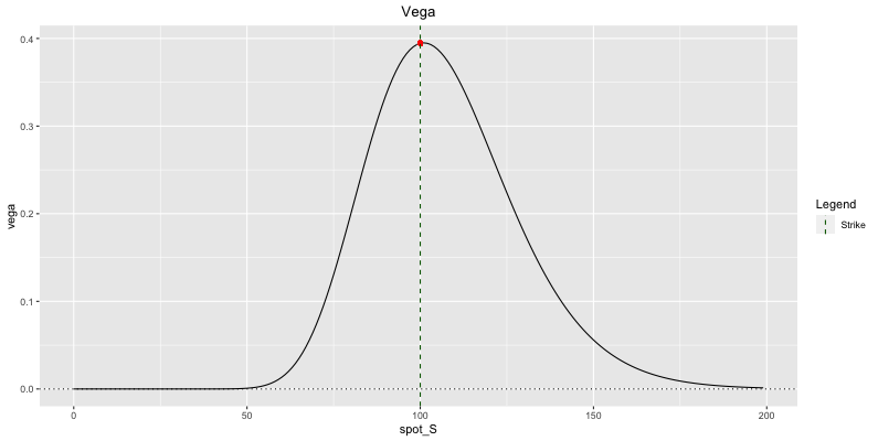
Fig: 5.14 : Call Vega
As for gamma, vega is greatest for ATM options and decays exponentially on both sides.
In fact, Gamma and Vega play a similar role to the options price.
Gamma is crucial to understanding how much money the hedge is making/losing. It was directly related to the realised volatility.
The Vega is in a way the forward measure for this.
Bell-Shaped Curve
The bell-shaped curve of vega makes sense intuitively.
When ATM, a change in the volatility can send the option either ITM or OTM thus the large effect on the price.
The vega sensitivity becomes really small when the option is either far ITM or far OTM because these options have already picked their direction in a way. A larger volatility won’t make that much difference to the price of the option. These kinds of options are quite easy to hedge, at least to the extent that when the market stays in the same regime, the hedge adjustments are minor over the lifetime of the option.
Of course there is a turning point, where the impact becomes stronger again. As soon as volatility is above this level, one could say the vega becomes meaningful, or the option is ATM from a vega point of perspective.
The shape of the curve is very similar to the shape of the normal density function, but within the expression of vega, there is an extra S factor that gives a twitch of bias.
5.5.4 Vega sensitivities
5.5.4.1 Moneyness
Vega generally has its peak value close to ATM and decreases as the option goes deeper ITM or OTM. Options that are deeply ITM/OTM have vega close to zero. This behavior is obvious when looking at figure 5.14.
5.5.4.2 Volatility
A higher volatility results in a wider vega curve, meaning a vega curve that is more flat. This points to the fact that in highly volatile markets the ATM point is less defined. The ATM region has become bigger.
Higher volatility does not necessarily mean higher vega in the ATM point!
The vega does not depend strongly on the level of volatility used, at least not once a certain critical level of volatility is reached.
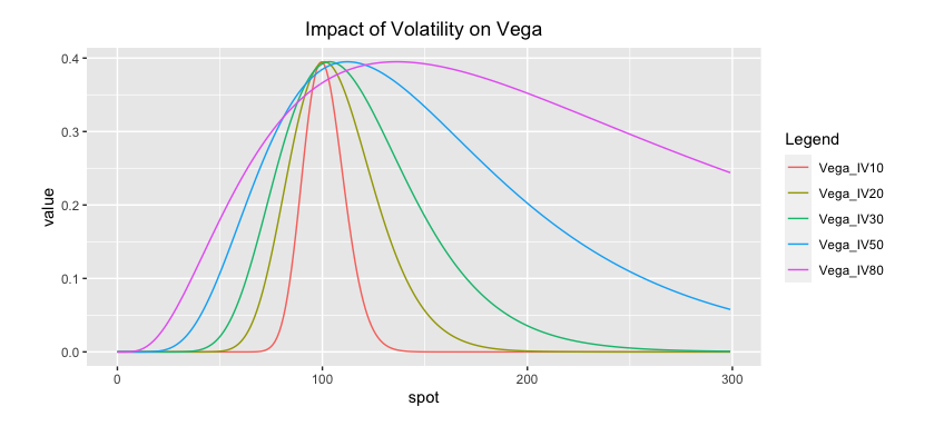
Fig: 5.15 : Impact of Volatility on Vega
5.5.4.3 Time to Maturity
We know that options lose their time value as time passes and we approach the expiry. It is not surprising that the volatility sensitivity or vega dies out.
Vega/Gamma have the same qualitative behaviour: largest ATM vs ITM/OTM. However, they have opposite dynamic behaviour: gamma spikes towards maturity whereas vega dies out!
If we want to capture forward volatility, then we have to trade options with the largest vega.
If we want to trade the spot volatility, then we have to trade options with largest gamma.
When the option is away from the strike levels, vega drops very quickly with time. Only ATM options can hold their vega for a longer time.
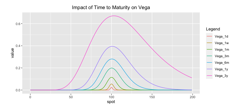
Fig: 5.16 : Impact of Time to Maturity on Vega
For more exotic structures, the vega profile can change sign, and whether we are short or long volatility depends on the underlying’s price.
The ATM option is almost linear in volatility.
The prices of the ITM and OTM options are convex in volatility up to a certain level then become linear for large volatilities.
5.6 Rho
5.6.1 Description
Rho represents the sensitivity of an option’s price to a movement in interest rates.
As the delta, it is positive for calls and negative for puts.
The prices of vanilla options are almost linear in interest rates. In other words, it only has a first-order effect. This effect comes from:
- the impact of interest rates on the cost of the delta-hedge.
- the discounting of the option price.
The second effect is generally smaller than the first one.
5.6.2 Calls
A trader sells a call option and delta hedges by buying delta shares. To buy those shares, he must borrow money at the bank. He will have to pay interest on his loan.
The higher the interest rates, the more interests to pay, the higher the cost of his hedge, the higher the call price. This is the reason why rho is positive for call options.
The discounting effect slightly offsets this delta hedge impact though. \(\boxed{\text{Call Rho} = \rho = \frac{\partial C}{\partial r} = K \; t \; e^{-rt}N(d_2)}\)
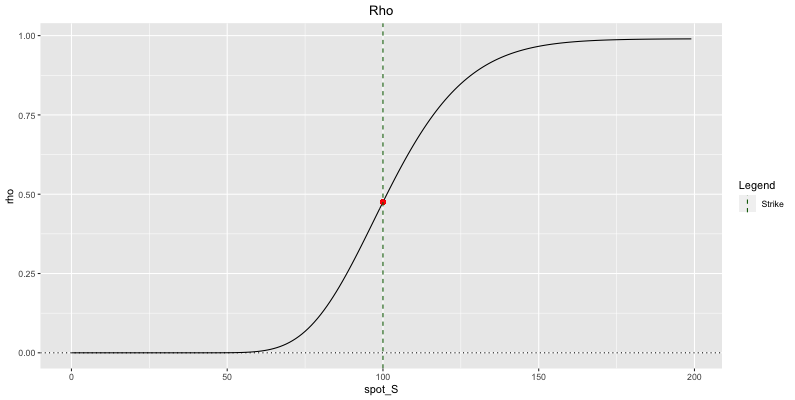
Fig: 5.17 : Call Rho
5.6.3 Puts
A trader sells a put option and delta hedges by selling delta shares. By selling shares, he receives money. He can put this money in the bank and receives interest on it.
The higher the interest rates, the more interests he receives, the lower the cost of his hedge, the less expensive the put price. This is the reason why rho is negative for put options.
The discounting effect works in the same direction and reinforces this impact.
If you make more money on your delta hedge, you are going to pay more (receive less) for it.
\(\boxed{\text{Put Rho} = \rho = \frac{\partial P}{\partial r} = -K \; t e^{-rt}N(-d_2)}\)
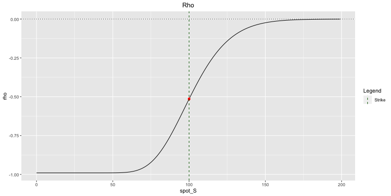
Fig: 5.18 : Put Rho
5.6.4 Rho sensitivities
5.6.4.1 Moneyness
Rho is larger for ITM options and decreases steadily as the option changes to become OTM.
5.6.4.2 Time to Maturity
Rho increases as time to expiration increases. Long-dated options are far more sensitive to changes in interest rates than short-dated options.
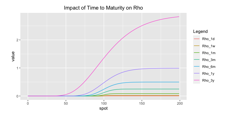
Fig: 5.19 : Impact of Time to Maturity on Rho
Though rho is a primary input in the Black-Scholes model, a change in interest rates generally has a minor overall impact on the pricing of options. Because of this, rho is usually considered to be the least important of all the option Greeks.
5.6.5 Rho Hedging
We recall from delta-hedging procedure that we were using a cash account, where we received/were charged an interest rate r, continuously compounded, meaning every day we would receive/pay interest.
This is a source of uncertainty.
One can expect that the interest received for cash is lower than the interest to be paid for a loan. This typical bid/offer spread in interest rate market is the first of our problems.
What’s next?
The interest rates are not constant. So we don’t know in advance what the applicable rate interest rate is.
If we have a certain amount on the cash account, we could fix the interest rates for the lifetime of the option, but only for this fixed volume.
Because of the dynamic nature of the hedging procedure, the cash on the account will constantly change and a few days later, the conditions in the market might have changed. So, the best we can do is fix as much as we can at the start of the procedure, where we have at least an accurate view on the money in the cash account. For the future, the trader will use an estimate of the future interest rates.
The problem of uncertain interest rates in the context of equity derivatives is sometimes handled by the bank by fixing an internal system.
5.6.5.1 Internal Markets
For the sake of making the point, we will oversimplify.
Suppose you have 2 different desks in a trading floor:
- The desk that trades options on stocks.
- The desk that trades interest rates.
This will allow the interest rate risk to be transferred from one desk to the other. The management could decide that an internal system needs to be set up to accommodate for this transfer.
Therefore management could decide that the equity derivatives desk always receives an interest rate \(r-∆r\) and pays an interest rate \(r+∆r\). The spread \(∆r\) could be fixed internally to whatever value is reasonable. Often \(∆r = 0\) as it is usually clear in advance if an activity will be drawing cash or is self-funding.
That just leaves the determination of r. The fixing of this is harder. Taking the overnight interest rate, which would be the closest match to what we are looking for, leaves out great opportunities.
A bank typically has a good view on the value of the cash account as it has built up some history over time. Leaving the cash on this account does not make sense. The equity desk should shift this capital to other desks where it can be invested and managed more wisely.
One could decide that, for internal purposes, the interest rate r is taken to be the 6-month swap rate, irrespective of option lifetime. One could even decide that value of r is fixed once a week and kept constant throughout the week.
That means that the internal transfer is obligated and, in some cases, the interest desk is forced to take on positions with a loss, at other times it could be a profit. If the volumes coming from the equity derivatives desk are much smaller than the typical volumes they trade, this might not be as bad as it sounds.
For the equity derivatives desk, it eliminates the burden of following up on interest rates.
If the activity is organized this way, it is clear that the equity desk could arbitrage the system. If the interest rate is fixed on Monday and valid until Friday and they are looking into a transaction on Friday, and the interest rate market has changed a lot, they could decide to keep their interest rate position open and wait to deposit the cash until next Monday. An internal check-up should be installed to prevent one-sided abuse between the internal desks.
The main conclusion to be drawn from this is that an equity derivatives trader should be less focused on the problem of interest rate risk, and more on the value of the stock, and, on the volatility.
In practice, desks don’t have a cash account but instead they receive internal funding.
This funding has become more and more a topic of discussion as the regulator has raised the question if banks have enough capital available to run their business. From the cost of hedging argument, it is clear that the cost of funding should be factored into the hedging cost and hence into the price of any derivative.
Different participants in the market will have different funding rates, depending on the capitalization and credit rating they have. This leads to different internal interest rates, but also to different option prices, which they can offer to their clients.

5.7 General Practical Example
Let us go through an example that explains the concept of vega-gamma-theta hedging.
Suppose we have a portfolio with the following Greeks representation:
- Delta = 300.000
- Gamma = 2.500
- Theta = -500.000
- Vega = 750.000
Let us assume the following market parameters: - Stock price = 1.500 - Interest rate r = 2.5% - Dividend yield q = 0% - Volatility = 25%
Is it possible to design a portfolio that would offset all the Greeks simultaneously?
Well, we can obviously eliminate delta without making a difference to any other Greeks by selling stocks.
To hedge out the other Greeks, we need to use instruments that have non-zero Greeks. In other words, we have to use options.
Let us assume we have 3 options available:
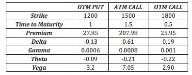
Fig: 5.20 : Table of available options
If we construct a portfolio with the following weights:
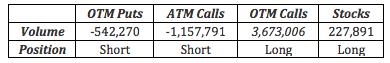
Fig: 5.21 : Weighted portfolio
How did we obtain these weights? Is it always possible to find those kinds of positions such that we get back what we want?
If we define the weights: \(w_1\), \(w_2\), \(w_3\), \(w_4\) respectively.
We are then trying to obtain a portfolio with portfolio Greeks equal to the ones we are after.
Mathematically speaking:
\(w_1\Delta_1 + w_2\Delta_2 + w_3\Delta_3 + w_4 = \Delta_V\) \(w_1\Gamma_1 + w_2\Gamma_2 + w_3\Gamma_3 = \Gamma_V\) \(w_1\Theta_1 + w_2\Theta_2 + w_3\Theta_3 = \Theta_V\) \(w_1v_1 + w_2v_2 + w_3v_3 = v_V\)
From basic linear algebra, this set of equations has a solution if its determinant is different from zero:
\[\begin{vmatrix}\Gamma_1 & \Gamma_2 & \Gamma_3 \\ \Theta_1 & \Theta_2 & \Theta_3 \\ v_1 & v_2 & v_3 \end{vmatrix} \neq 0\]
As it turns out, if we try to use 3 options with identical maturities, this determinant gets to be very close to zero. The reason for this is of course that all options are similar derivatives on the same instrument and the relationship between the Greeks makes the difference between using one option or three options very small. In other words, these options are not independent enough to build up an arbitrary portfolio.
A good mix of strikes and maturities solves this problem.
In the above example, we were looking for the hedging portfolio. If we put on this hedge, it is typically still a dynamic hedge that will need to be adjusted as market moves. But because we minimised more Greeks, the hedge is more stable and rebalancing won’t have to happen as often. It becomes much more of a semi-static hedge. If we have more options available, we can minimise more Greeks and make it an even better hedge.
One can prove that if we are trying to hedge an exotic derivative whose payout is only determined by the terminal value \(S_T\), then there exists a static hedge, provided we can use all the different strikes.
In practice, one can build a portfolio with features that the trader finds desirable: long vega and short gamma for example.
This portfolio exercise is the foundation for vega, gamma and theta trading.
5.8 Second-Order Greeks
5.8.1 Volga
Vega–Gamma, or Volga, is the second-order sensitivity of the option price to a movement in the implied volatility of the underlying asset.
\(\boxed{Volga = \frac{\partial^2 V}{\partial \sigma^2} = \frac{\partial v}{\partial \sigma}}\)
When an option has such a second-order sensitivity we say it is convex in volatility, or has vega convexity.
ITM and OTM European options do exhibit vega convexity but these can be captured in the skew.
Other structures exhibit a lot of vega convexity and will result in losses if we do not use a model that prices this correctly. The reason is that as volatility moves, a vega convex payoff will have a vega that now moves with the volatility and this must be firstly priced correctly and then hedged accordingly.
5.8.2 Vanna
Vanna measures the sensitivity of the option price to a movement in both the underlying asset’s price and its volatility.
\(\boxed{Vanna = \frac{\partial^2 V}{\partial S \partial \sigma} = \frac{\partial v}{\partial S} = \frac{\partial \Delta}{\partial \sigma}}\)
We can thus think about vanna as:
- the sensitivity of the option’s vega to a movement in the underlying’s price.
- the sensitivity of an option’s delta to a movement in the volatility of the underlying.
As such, vanna gives important information regarding a delta hedge by telling us by how much this delta hedge will move if volatility changes. It also tells us how much vega will change if the underlying moves. It can thus be important for a trader who is delta or vega hedging.
If vanna is large, then the delta hedge is very sensitive to a movement in volatility.
5.8.3 Charm
Charm, or delta decay, is the rate at which the delta of an option changes with respect to time. It refers to the second order derivative of an option’s value, once to time and once to delta.
\(\boxed{Charm = \frac{\partial \Delta}{\partial t} = - \frac{\partial \Delta}{\partial T} = \frac{\partial \Theta}{\partial S} = - \frac{\partial^2 V}{\partial S \partial T}}\)
Charm values range from -1 to +1.
As time passes, the option loses more of its time value, OTM options see their delta approach zero and ITM options see their delta become closer to that of an equivalent position in the underlying. In other words, each day that passes, OTM options require less delta hedging, and ITM options require more.
- Positive Charm: ITM calls and OTM puts.
- Negative Charm: ITM puts and OTM calls.
- Zero Charm: ATM options.
I personally haven’t dealt much with this second-order greeks but it is particularly relevant for options traders. They must indeed pay close attention to their charm on Friday. At that moment, the market closes for more than two days and the charm’s effect is magnified and impacts their options action on Monday. Paying attention to the charm may prevent the trader from over or under hedging. Special attention is needed around a charm’s expiration time, as it may become very dynamic.
5.9 Multi-Asset Greeks
5.9.1 Cross-Gamma
The cross-Gamma is the sensitivity of a multi-asset option to a movement in two of the underlying assets. The cross Gamma involving \(S_i\) and \(S_j\) is given by:
\(\boxed{\Gamma_{i,j} = \frac{\partial V^2}{\partial S_i \partial S_j} = \frac{\partial \Delta_i}{\partial S_j} = \frac{\partial \Delta_j}{\partial S_i}}\)
It is the effect of a movement in \(S_i\) on the delta sensitivity of the option to \(S_j\).
In multi-asset options, gammas could be expressed in a matrix form, with elements on the diagonal being gammas and elements off the diagonal being cross gammas.
In multi-asset options, it is possible that the delta with respect to one asset can be affected by a movement in another underlying asset even if the first asset has not moved.
5.9.2 Cega = Correlation Delta
The correlation delta is the first-order sensitivity of the price of a multi-asset option to a move in the correlations between the underlyings.
The correlation delta with respect to assets \(S_i\) and \(S_j\) is given by:
\(\boxed{Cega_{(i,j)} = \frac{\partial V}{\partial \rho_{i,j}}}\)
In the contest of pricing derivatives with multi-assets, we measure the degree of the dependence or dispersion of multi-assets through the correlation matrix.
Correlations vary over time. A multi-asset product’s sensitivity to the correlation between a pair of underlying assets can vary as the other parameters change.
While correlation is not easily tradable, there are some methods of trading correlation. Many correlation risks are not completely hedgeable, if at all, and in many cases traders must resort to maintaining dynamic margins for the unhedged correlation risk. Knowing the sign and magnitude of correlation sensitivity is again necessary in this case.
Some multi-asset derivatives are convex in correlation, meaning that the second-order effect on the price from a movement in the correlation is non-zero and needs to be taken into account.
5.10 Computational Methods
There are many different ways to compute the greeks, but we will focus on 3 popular methods:
- Finite-difference approximations
- Pathwise method
- Likelihood Ratio method
5.10.1 Finite-difference approximations
They involve calculating the price for a given value of a parameter, then changing the parameter value slightly, by \(\epsilon\), and recalculating the price.
Let \(f\) be the payoff function and \(\theta\) the parameter we are interested in.
Forward difference method
An estimate of the sensitivity will be: \(\boxed{\Delta = \frac{f(\theta \ + \ \epsilon) \ - \ f(\theta)}{\epsilon}}\)
Backward difference method
An estimate of the sensitivity will be: \(\boxed{\Delta = \frac{f(\theta) \ - \ f(\theta \ - \ \epsilon)}{\epsilon}}\)
Central difference method
An estimate of the sensitivity will be: \(\boxed{\Delta = \frac{f(\theta \ + \ \epsilon) \ - \ f(\theta \ - \ \epsilon)}{2 \epsilon}}\)
Advantages and Disadvantages
Advantages
- It is easy to implement and does not require too much thought.
- Monte Carlo simulation can be used.
Disadvantages
- It is a biased estimator of the sensitivity.
This is reduced by using the central difference method. However, this method is slower as there are three prices to calculate.
- There is an issue with discontinuous payoffs.
Let us explain further this last disadvantage using a specific discontinuous payoff such as a Digital Call.
If we want to estimate the delta of a digital call, we will get it being zero except for the few times when it will be 1. For these paths, our estimate of delta will be very big, approximately of order \(\epsilon^{-1}\).
5.10.2 Pathwise method
It gets around the problem of simulating for different values of \(\theta\) by first differentiating the option’s payoff and then taking the expectation under the risk-neutral measure:
\(\boxed{\Delta = e^{-rT} \; \int \frac{\theta_T}{\theta_0} f^{'}(\theta_T) \ \Phi(\theta_T, \theta_0) \ d\theta_T}\)
Where \(\Phi\) is the density of \(\theta\) in the risk-neutral measure.
Advantages and Disadvantages
Advantages
- It is an unbiased estimate.
- It only requires simulation for one value of \(\theta\) and is usually more accurate than a finite-difference approximation.
Disadvantages
It becomes more complicated when payoff is discontinuous. To get around this we can rewrite f = g + h, with g being continuous and h piecewise constant.
5.10.3 Likelihood ratio method
Similar to the pathwise method, but instead of differentiating the payoff we differentiate the density \(\Phi\):
\(\boxed{\Delta = e^{-rT} \int f(\theta_T) \frac{\Psi}{\Phi}(\theta_T) \Phi(\theta_T) \ d\theta_T}\)
Where \(\Psi\) is the derivative of \(\Phi\) by \(\theta\).
Advantages and Disadvantages
Advantages
- Only one value of \(\theta\) needs to be simulated to calculate both the price and the sensitivity.
- There is no need to worry about discontinuities in the payoff function as we are differentiating the density.
Disadvantages
The density needs to be explicitly known.
