1
Prerequisites
2
Introduction to the Structured Products Market
2.1
The Structured Products
2.1.1
Introduction
2.1.2
Issuing Wrappers
2.2
The Stakeholders
2.2.1
The Sell Side
2.2.2
The Buy Side
3
Back to Basics!
3.1
Interest Rates
3.1.1
Introduction
3.1.2
LIBOR and Treasury rates
3.1.3
Yield curves
3.2
Bonds
3.2.1
Introduction
3.2.2
Market Price
3.2.3
Bonds’ underlying risks
3.2.4
Zero-Coupon bonds (ZCB)
3.3
Equities
3.3.1
Dividends
3.3.2
Repurchase Agreement (Repo)
3.3.3
Liquidity
3.4
Forwards and Futures
3.4.1
Introduction
3.4.2
Delivery price, Forward price and Forward value
3.4.3
Forward price of a stock
3.5
Swaps
3.5.1
Interest Rate Swaps (IRS)
3.5.2
Cross-Currency Swaps (CCS)
3.5.3
Total Return Swaps (TRS)
3.5.4
Dividend Swaps
3.6
Options
3.6.1
Introduction
3.6.2
Call Options
3.6.3
Put Options
4
A deeper understanding of Options
4.1
The Black-Scholes model
4.1.1
Risk-Neutral Pricing
4.2
European Call Options
4.2.1
Introduction
4.2.2
Buyer’s payoff at maturity
4.2.3
Market Price or Premium
4.3
European Put Options
4.3.1
Introduction
4.3.2
Buyer’s payoff at maturity
4.3.3
Market Price or Premium
4.4
Intrinsic Value and Time Value
4.4.1
Introduction
4.4.2
Time Value of Call Options
4.4.3
Time Value of Put Options
4.5
The Cost of Hedging
4.6
The Call-Put Parity
4.6.1
Introduction
4.6.2
The Call-Put relationship
5
The Greeks
5.1
Introduction to the Greeks
5.1.1
Introduction
5.1.2
Taylor Series
5.1.3
Static and Dynamic Hedge
5.1.4
Summary Table of the Greeks
5.2
Delta
5.2.1
Description
5.2.2
Calls
5.2.3
Puts
5.2.4
Assets to delta hedge
5.2.5
Delta under Black-Scholes
5.2.6
Delta sensitivities
5.2.7
Other factors linked to delta hedge
5.2.8
Delta as a hedge ratio, not a probability
5.2.9
Setting up a small delta-hedging experiment
5.3
Gamma
5.3.1
Description
5.3.2
Gamma under Black-Scholes
5.3.3
Gamma sensitivities
5.3.4
Negative Gamma at maturity is tricky
5.3.5
Gamma P&L
5.3.6
An example
5.3.7
Can volatility be captured by delta-hedging?
5.3.8
Dollar Gamma
5.4
Theta
5.4.1
Description
5.4.2
Theta under Black-Scholes
5.4.3
Some features of Theta
5.4.4
Gamma and Theta are always flirting
5.5
Vega
5.5.1
Description
5.5.2
The Vega Matrix
5.5.3
Vega in the Black-Scholes model
5.5.4
Vega sensitivities
5.6
Rho
5.6.1
Description
5.6.2
Calls
5.6.3
Puts
5.6.4
Rho sensitivities
5.6.5
Rho Hedging
5.7
General Practical Example
5.8
Second-Order Greeks
5.8.1
Volga
5.8.2
Vanna
5.8.3
Charm
5.9
Multi-Asset Greeks
5.9.1
Cross-Gamma
5.9.2
Cega = Correlation Delta
5.10
Computational Methods
5.10.1
Finite-difference approximations
5.10.2
Pathwise method
5.10.3
Likelihood ratio method
6
All about Volatility
7
Classic Options
8
Options Strategies
9
Asian Options
10
Quanto Options
11
Compo Options
12
Barrier Options
13
(Barrier) Reverse Convertibles
14
Certificates
15
Multi-Asset Options
16
Autocallables
17
Variance Swaps
The Derivatives Academy
Chapter 12
Barrier Options
You can
register
to get access to the
FULL ebook and the associated pricers!
Chapter 12 - Barrier Options: Overview
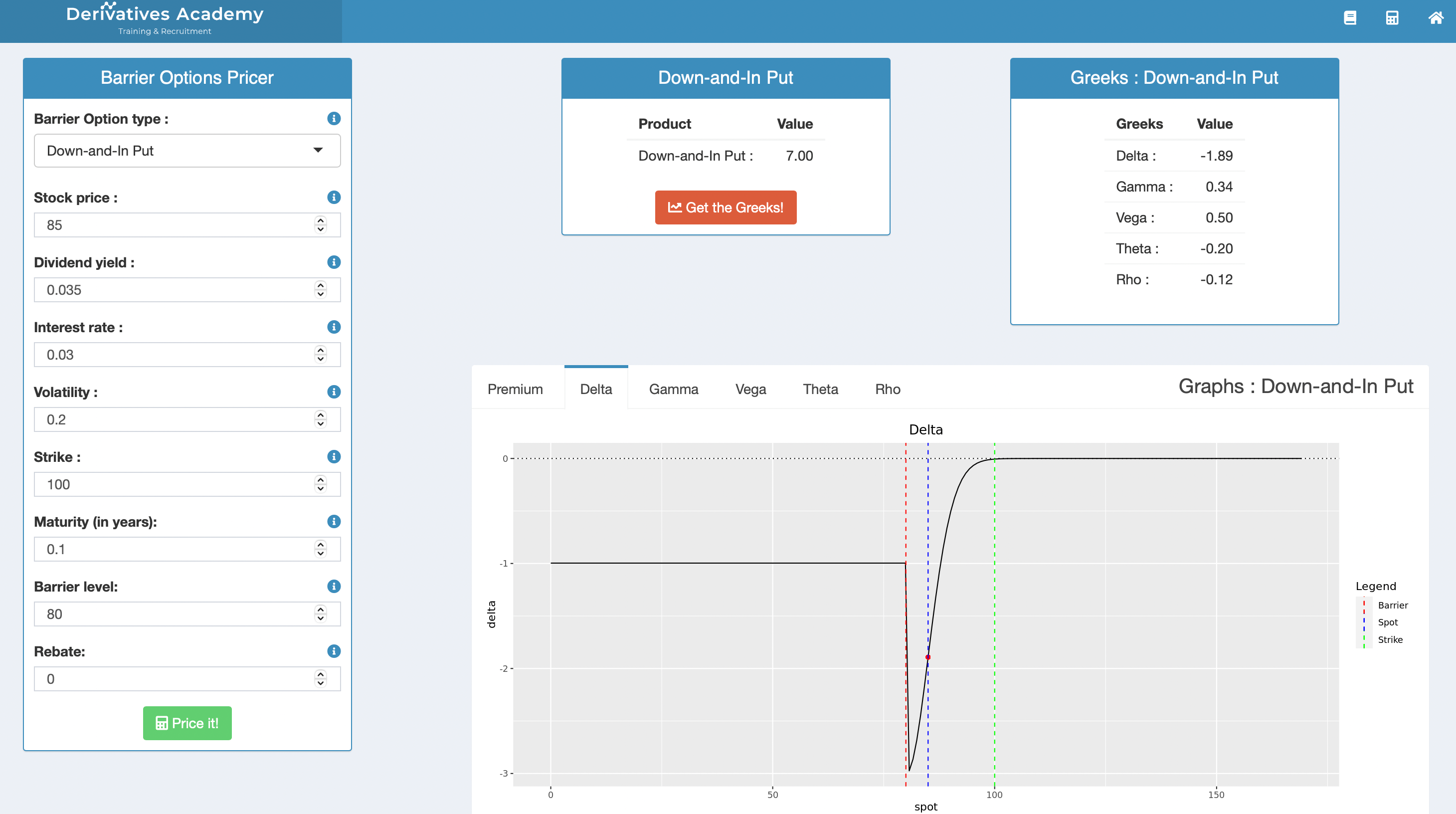
Chapter 12 - Barrier Options: Pricer
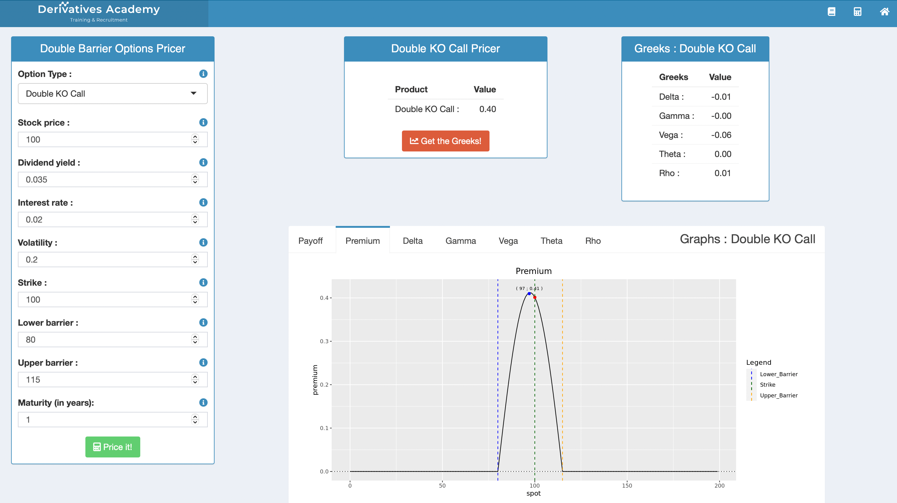
Chapter 12 - Double Barrier Options Pricer