Section 4 Model results

4.1 Model output

The input data for the model was obtained from the fluxnet site at Hainich for the year 2018.

The first step is exploring the main model output both for the shortwave and longwave component.

4.1.1 Shortwave

The shown shortwave variables are:

Incoming sw (measured) \(I^\downarrow\)
Absorbed sw by canopy \(I^\uparrow\)
Upward sw reflected by the canopy \(\overrightarrow{I}_{c}\)
Absorbed sw soil \(\overrightarrow{I}_{g}\)

Due to radiative balance those variables are in the following relationship:

\(I^\downarrow = I^\uparrow + \overrightarrow{I}_{c} + \overrightarrow{I}_{g}\)

One week

In figure 4.1 the model output for the shortwave is plotted for one week during the summer. The daily cycle can be clearly seen, with all variables having a peak at noon and reach the value of \(0\) during the night. The total incoming radiation changes depending on the day, mainly due to cloud cover, and the absorbed shortwave follow its pattern.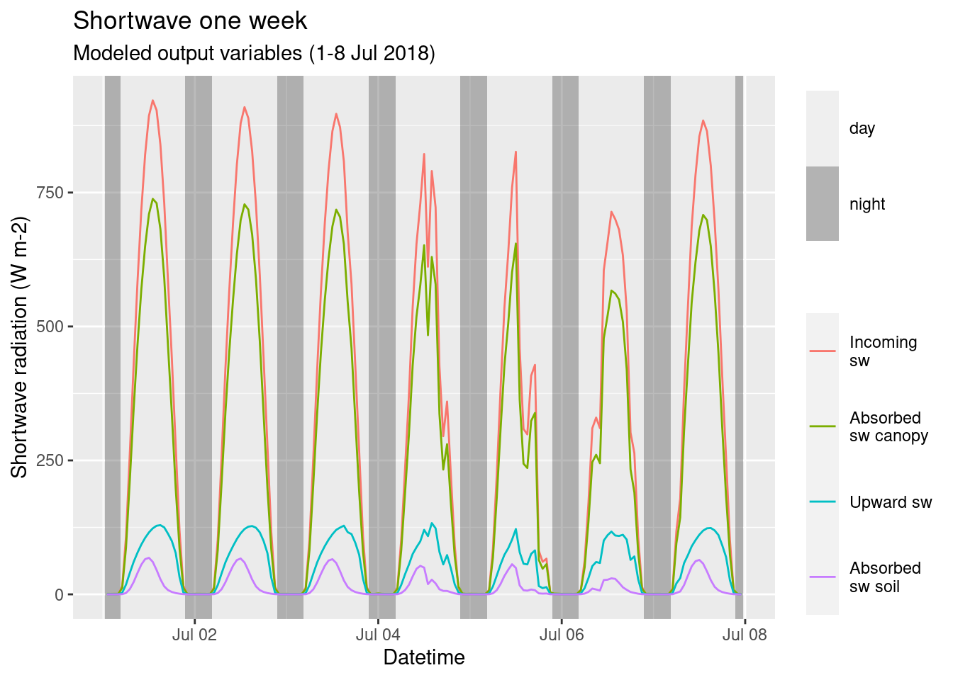

Figure 4.1: Shortwave one week. Modeled output variables (1-8 Jul 2018).

One year

Then the shortwave over one year is analyzed (Figure 4.2), after averaging over one week. There is a yearly cycle in the incoming shortwave radiation with a significant difference, as the averages goes from more than \(300 W m^2\) to almost \(10 W m^2\) (this is the week average so takes into account also the night when shortwave radiation is zero).

The absorbed by the soil depends on the amount of LAI, in fact during the spring when the radiation is high but there are no leaves yet its values increase constantly. As soon as leaves starts to come out the shortwave absorbed by the soil decreases to reach a stable low value during the summer and eventually increase again when leaves fall.

The radiation reflected by the canopy doesn’t have a big change over the year and overall canopy albedo remains for the all year between \(0.16\) and \(0.20\). Finally, the radiation absorbed the canopy follows, as expected, the pattern in the incoming radiation. During the spring its value are really similar to the shortwave absorbed by the soil, however this is only a coincidence.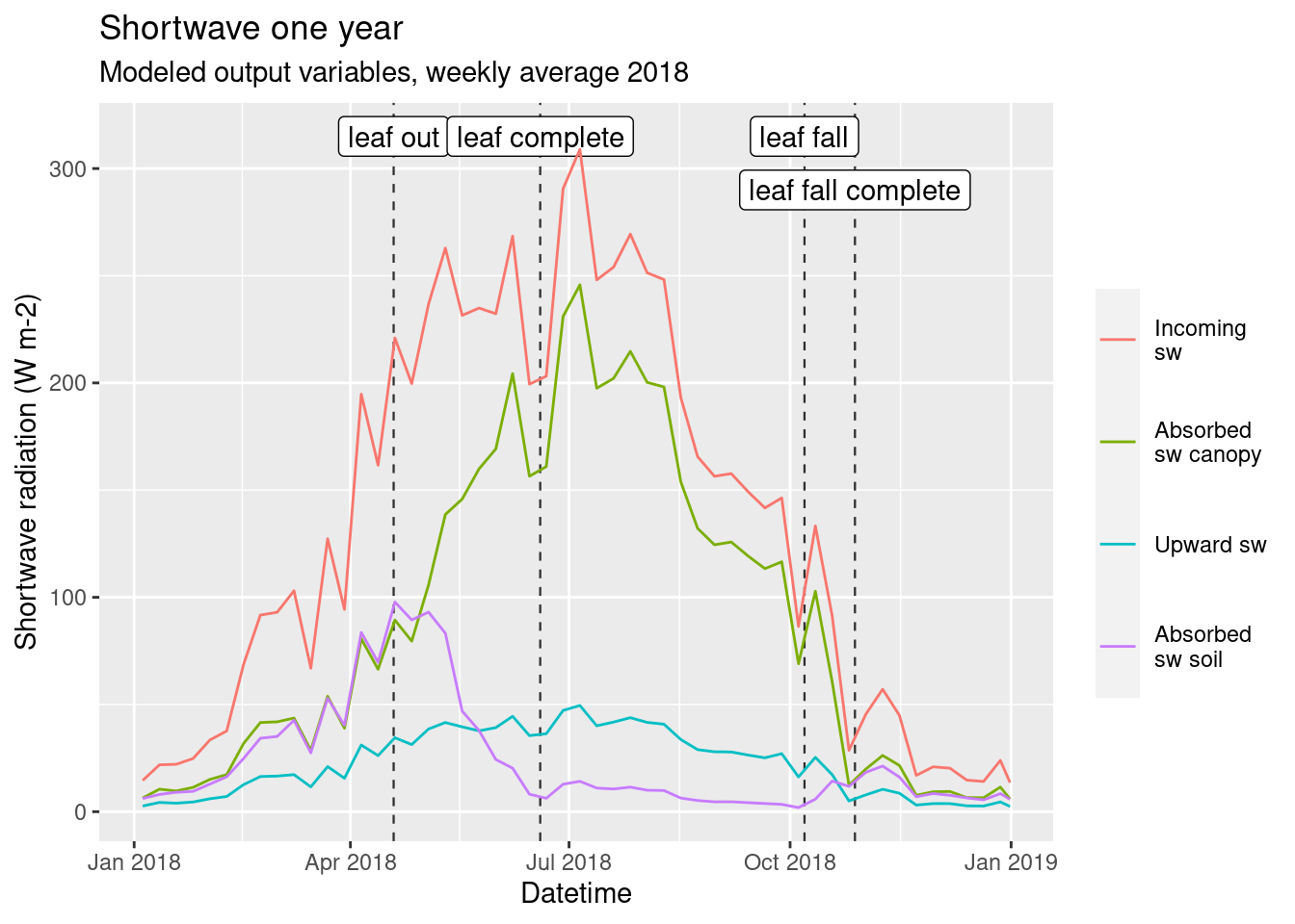

Figure 4.2: Shortwave one year. Modeled output variables, weekly average 2018. Vertical black lines are the moment when there is change in LAI

4.1.2 Longwave

The shown longwave variables are:

Incoming lw (measured) \(L^\downarrow\)
Absorbed lw by canopy \(L^\uparrow\)
Upward lw emitted by the canopy \(\overrightarrow{L}_{c}\)
Absorbed lw soil \(\overrightarrow{L}_{g}\)

Due to radiative balance those variables are in the following relationship:

\(L^\downarrow = L^\uparrow + \overrightarrow{L}_{c} + \overrightarrow{L}_{g}\)

One week

Longwave radiation haa a daily cycle, but the variation is much smaller compared to shortwave (Figure 4.3). The canopy is emitting more longwave radiation than the one that is receiving from the sky, hence the absorbed radiation from the canopy is negative. The incoming shortwave radiation depends on the weather, with cloudy skies resulting in higher level of incoming radiation as it can be seen on the 5-6 of July. The difference can be quite important with an increse of about 30% in radiation levels. The upward longwave radiation, instead, depends on the temperature of the canopy and the soil, which is influenced by heat fluxes and shortwave radiation. Therefore, the incoming and outgoing radiation don’t change together, hence there is a variation the radiative balance. In fact it almost reaches zero in the morning of the 6th of July.

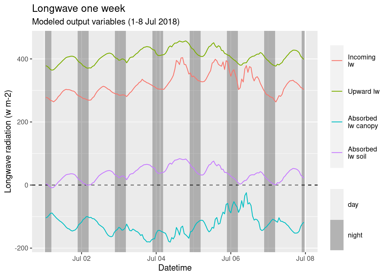
Figure 4.3: Longwave output over one week

One year

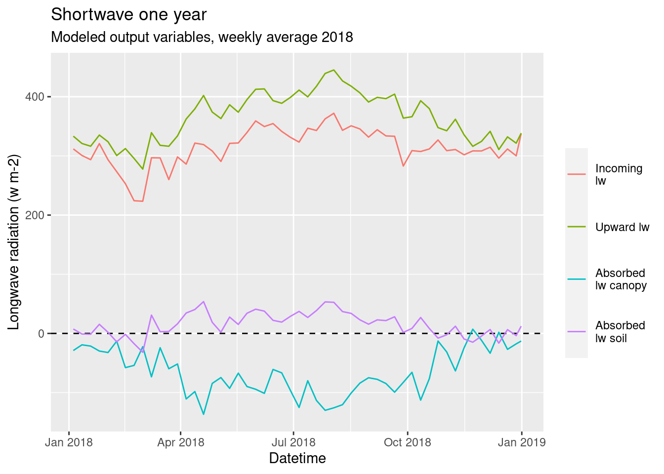
During the year there longwave radiation has a cycle with higher values in the summer than in the winter. The difference is, however, limited between seasons. In general the behaviour is comparable with the 1 week period.

4.2 Model evaluation

The model results are compared with observed data to evaluate the model accuracy. It is done independently for the longwave and shortwave components.

In the Hainich dataset there are observed variables that will be used for the evaluation.

The evaluation will be carried out by visually comparing time series and by quantitative means.

4.2.1 Shortwave

For the shortwave the only observed variable that can be used for the model evaluation is the outgoing shortwave radiation.

Time series

One Week

The model has an overall good agreement between the modeled outgoing shortwave, and the measured one (Figure 4.4).

The day peak of the model is often delayed compared to the observed one. This phase shift may connected to the relative long time interval (1 hour) in model outputs. The model generally slightly underestimates the radiation during sunny days (first 3 and last), while overestimates during with cloudy conditions. During the night the observed radiation is slightly above zero, while the model is at zero. This is clearly a measurement error, as during the night there is no shortwave radiation.

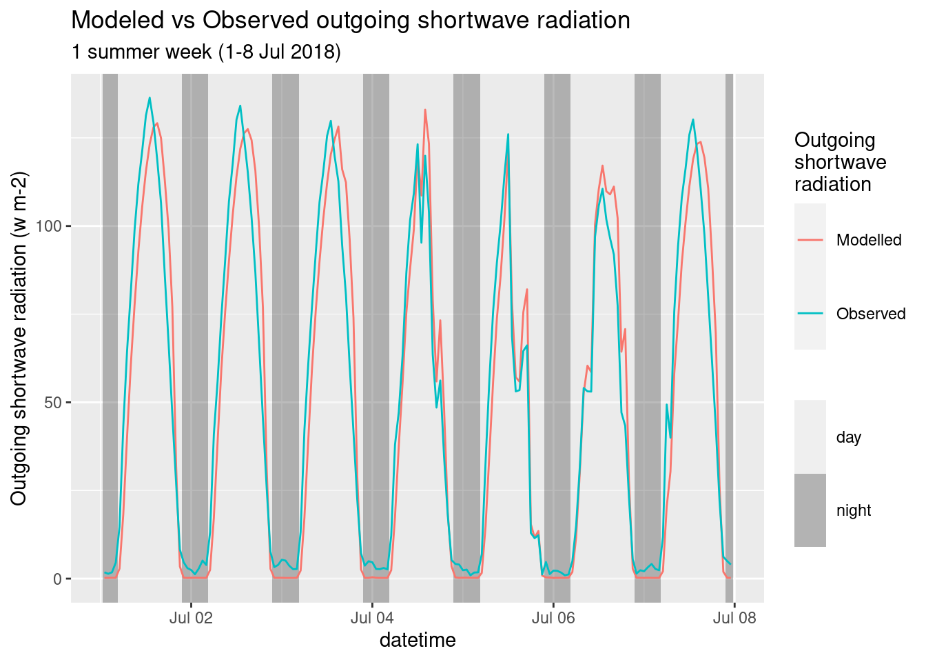
Figure 4.4: Shortwave Modeles vs Observed. One week.

One Year

By analyzing a model output over the whole year, there is a good overall performance (Figure 4.5). During spring, and partially during autumn, there is the biggest difference between the model output and the observations. This is probably connected to the fact that in that period the LAI is estimated with a simple linear equation, thus does not reflect completely the real world conditions.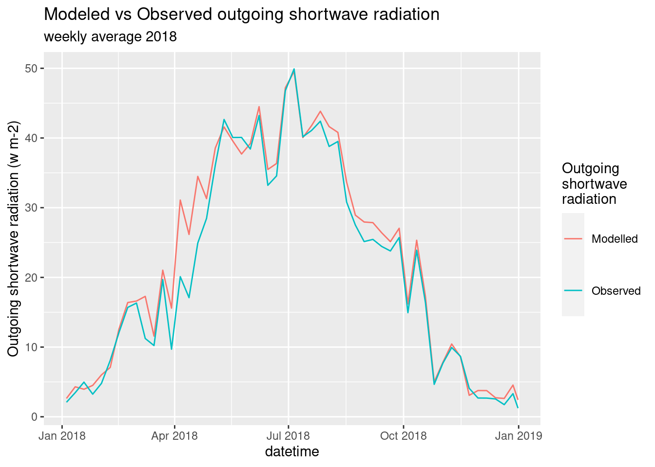

Figure 4.5: Shortwave Modeles vs Observed. One year.

Quantitative evaluation

The performance of the model has been also analyzed in a quantitative way. A linear model has been built between the observations, and the model output (Figure 4.6), if the model matched perfectly the observations the slope should be \(1\), the intercept \(0\) and the \(r^2 1\).

The results of the linear model are:

slope: \(0.87\)
intercept: \(1.38\)
\(r^2\): \(0.93\)

The intercept is really close to \(0\), and the slope and \(r^2\) also indicate a good fit.

The performance of the model has been also evaluated using the Root Mean Square Error (RMSE) and the Nash-Sutcliffe coefficient (NSE). The obtained values are:

RMSE: \(9.51\)
NSE: \(0.91\)

The NSE has a value of \(1\) when there is a perfect model and \(0.91\) can be considered really good. The RMSE can be interpreted as the amplitude of the error and compared to the range of the radiation. Therefore, in this scenario RMSE of \(9.51\) can be considered good but not perfect.

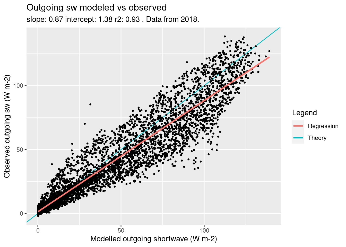
Figure 4.6: Modeled vs Observed outgoing sw, scatter plot

4.2.1.1 Conclusion

The performance of the model in more than satisfactory and the some of deviation from the observation can be explained with the inaccurate input data.

4.2.2 Longwave

In the same way of shortwave the only observed variable that can be used for the model evaluation is the outgoing longwave radiation.

Time series

One Week

The longwave components is also accurately modeled (Figure 4.7).

There is a daily pattern in the difference between the modeled and the observed outgoing longwave. This is probably due to the fact that the model doesn’t use the true leaf temperature, as it needs to be calculated by other models, but uses the air temperature as a proxy.

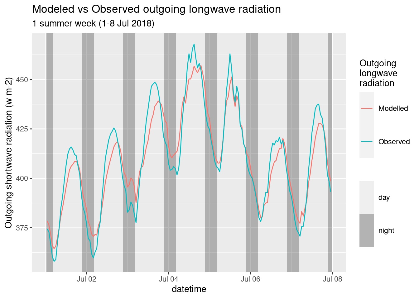
Figure 4.7: Longwave Modeles vs Observed. One week.

One Year

By comparing the week averages over the year (Figure 4.7) the model produces almost perfect output for the whole year.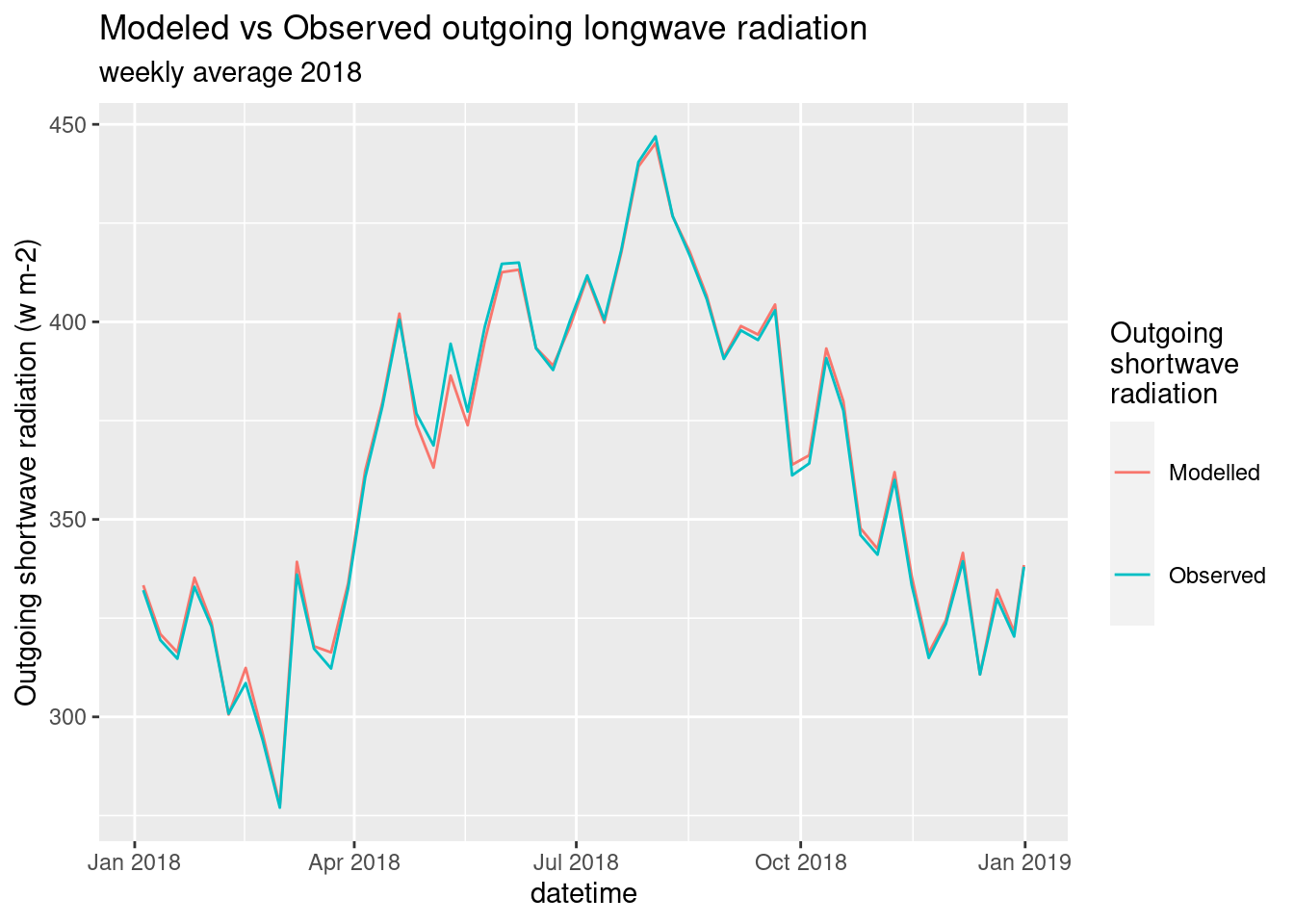

Figure 4.8: Longwave Modeles vs Observed. One year.

Quantitative evaluation

The same procedure for shortwave has been followed for the longwave of the quantitative evaluation of model performance.

The longwave model has a very good performance (Figure 4.9) The results of the linear model are:

slope: \(1.03\)
intercept: \(-11.09\)
\(r^2\): \(0.99\)

Both the slope and the \(r2\) have a value of \(1\) when rounded at the first decimal digit.

This is confirmed by the high value of the Nash-Sutcliffe coefficient and the low Root Mean square error:

RMSE: \(5.33\)
NSE: \(0.99\)

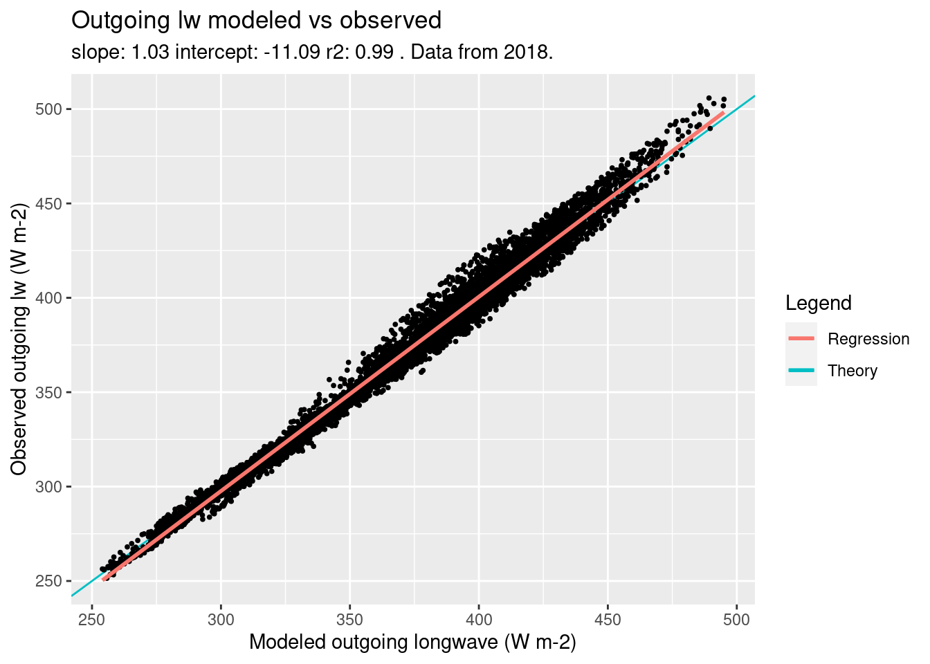
Figure 4.9: Modeled vs Observed outgoing lw. scatter plot

4.2.2.1 Conclusion

The longwave model performs very well. This is true in spite of the inaccurate leaf temperature that is used as input.