9 Calculating Network Size and Density

Now that we have a list of networks, we can apply the same function to each network using a single line of code, again with the help of lapply. Network size is the number of nodes in a network. To find this, we use the vcount() function. We can also find the number of edges using ecount()

network_sizes <- lapply(ego_nets, vcount)
network_edge_counts <- lapply(ego_nets, ecount)

head(network_sizes)

## [[1]]
## [1] 0
## 
## [[2]]
## [1] 0
## 
## [[3]]
## [1] 4
## 
## [[4]]
## [1] 4
## 
## [[5]]
## [1] 0
## 
## [[6]]
## [1] 5

We can take the mean of one of these results simply by turning the list into a vector and using the mean function on the resulting vector.

network_sizes <- unlist(network_sizes)
mean(network_sizes, na.rm = T)

## [1] 1.796634

The average network has a little over one and a half people in it. We could similarly plot the distribution.

hist(network_sizes, main = "Histogram of Ego Network Sizes", xlab = "Network Size")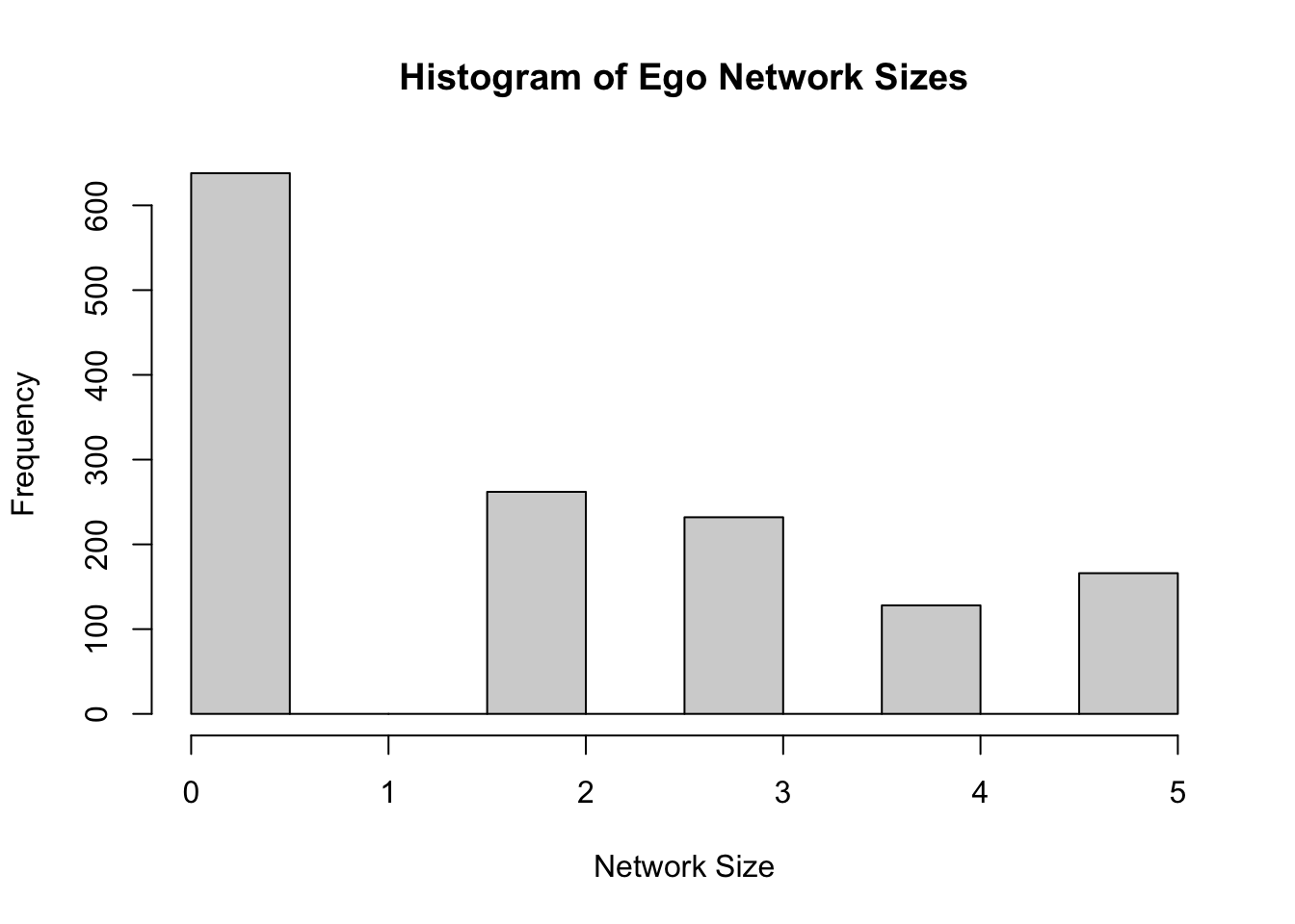

And, naturally, we can do the same for edges.

network_edge_counts <- unlist(network_edge_counts)
hist(network_edge_counts, main = "Histogram of Ego Network Edge Counts", xlab = "# of Edges")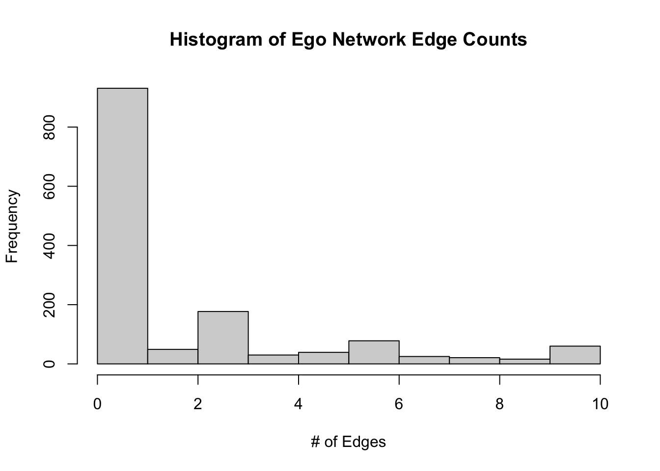

Finally, let’s try density. Density captures how many edges there are in a network divided by the total possible number of edges. In an undirected network of size N, there will be (N * (N-1))/2 possible edges. If you think back to the matrix underlying each network, N * N-1 refers to the number of rows (respondents) times the number of columns (respondents again) minus 1 so that the diagonal (i.e. ties to oneself) are excluded. We divide that number by 2 in the case of an undirected network only to account for that fact that the network is symmetrical.

We could calculate this on our own for the random ego network from before as follows.

ecount(random_ego_net)/((vcount(random_ego_net) * (vcount(random_ego_net) - 1))/2)

## [1] 0.6

igraph has its own function - graph.density which we can again apply to every ego network in the data.

densities <- lapply(ego_nets, graph.density)
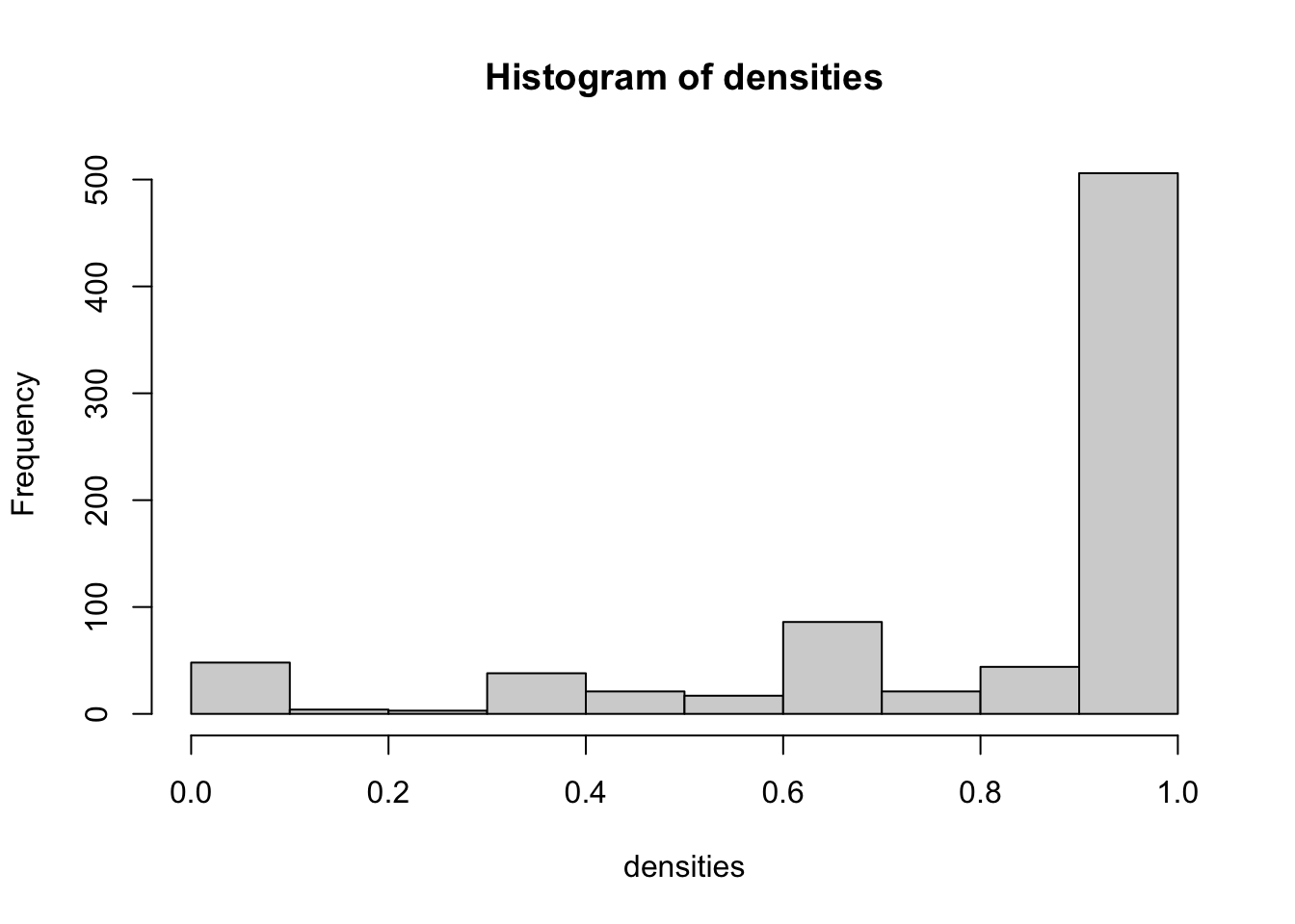
densities <- unlist(densities)

To end the tutorial, let’s plot the distribution of density across the different ego networks.

hist(densities)