8 Collecting and Merging Data
8.1 Collecting Data
For the final project in this class you are to find your own data and to generate a short presentation and blog post. The first step in this process is going to be looking for your own data.
This is going to be an iterative process. That is: you aren’t likely to just go out and grab the right data on the first pass. You are going to have to think about your area of inquiry, then look for data, refine your area of inquiry based on the data thats available, think about adding data based on this new question etc.
For this process keep in mind that we are here to help! We really want you to come to office hours to talk to us about what you are looking for and what problems you are facing. We’ve been doing this for awhile and can help you think through things if you hit dead ends, or to suggest extra data to supplement what it is that you are finding. Please come talk to us!
The remainder of this section will go over some guidelines for looking for data and some places to go and find it. The second section of this chapter deals with the critical step of merging two datasets together: the functions we use to combine two datasets that have common units of analysis.
8.1.1 What to look for?
To start off with: I would not encourage your first step to be to look for a dataset.
The first thing you should be doing is thinking about a realtionship in terms of concepts and not measures. What do I mean by this?
Let’s take a look at this graph I generated from American National Election Study looking at the relationship between the self-reported 7-point ideology measure and family income.
anes <- rio::import("https://github.com/marctrussler/IIS-Data/raw/main/ANES2020Clean.csv")

boxplot(anes$income ~ anes$ideology7, xlab="Ideology",
        ylab="Reported Family Income (Thousands)", outline=F, axes=F)
axis(side=2)
axis(side=1, at=1:7,
     labels=c("Very Liberal","2","3","4","5","6","Very Conservative"), cex.axis=0.8)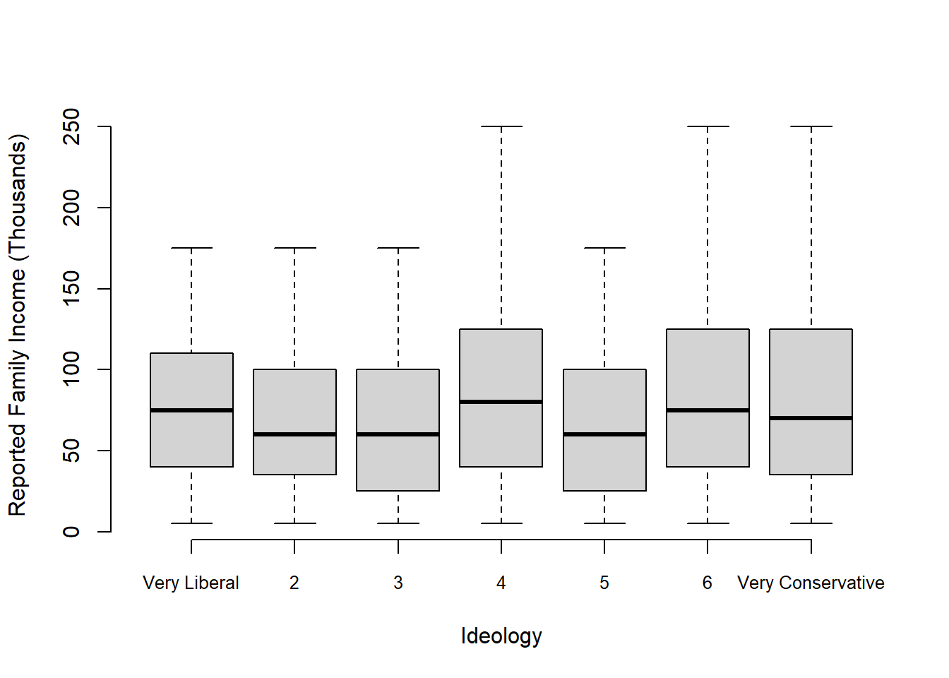
How should we describe the question this graph is answering?
We could say: What is the relationship between self reported 7-point ideology measures and reported family income?
But that’s pretty unsatisfying! We don’t really want to answer questions about questions in the ANES, we are interested in the broader concepts that these things represent. The question we actually want to answer is:
What is the relationship between ideology and wealth?
Asking the question this way makes us (1) think about what we really care about; and (2) forces us to grapple with the question: how well do these things measure the concepts we care about?
“Ideology” is a concept about how people think politics and society should be organized. The labels “liberal” and “conservative” are an interpretation of these fundamental positions, and the facto of putting it on a 7 point scale is a further abstraction that assumes a single dimensional scale. This may, or may not, do a good job of capturing the concept (lots of evidence suggests it does not), but at the very least, explicitly defining this as a measure makes us think about and defend this choice.
Indeed, even something basic like “family income” may or may not capture the concept of “wealth” correctly. This doesn’t take into account assets, investments, or generational wealth in a way that may matter for fully capturing this concept.
So: the first step in thinking about what sort of data you want to get is to think about the concepts you want to explore, and what sort of measures may do a good job in representing these concepts.
As I said before, this is going to be an iterative process. It’s nice to start with an ideal world: these are the measures that would perfectly represent my concept. But this will also happen backwards: redefining the concepts you are interested in based on the real world measures that are available.
Once you have your concepts you wish to measure the next step is to think through which unit of analysis you expect these things to be measured on.
To take our above example of “What is the relationship between ideology and wealth?” For this question we pretty much have to use individual data. We can measure wealth, at say, the county level, but it’s hard to measure ideology at that level. What is the collective ideology of Philadelphia? (Such measures actually exist, but the point remains that ideology is really thought of as an individual concept.)
But if our question was: “How did COVID-19 affect voter turnout?” this might be a question that is answered with aggregate data. We can measure COVID-19 exposure by the number of cases at the county level, and also measure voter turnout using election results at the county level. That being said, this relationship could also be answered at the individual level: measuring COVID exposure through self-reports of infection and voter turnout through self-reported turnout.
So sometimes the question you are answering forces you into a particular unit of analysis, and sometimes it allows you to make a choice. How should you think about those choices?
Individual data is often great when you can find it, and gives us the opportunity to look at more specific attitudes and behaviors that can only really be captured at the individual level. However, individual survey data is expensive! The National Exit Poll, which we help to administer at NBC, costs several million dollars. So with individual data you are limited to what other people have collected and made available. Further, most survey data is meant to be representative at the national or state level. It’s hard to get enough people in different counties to be representative. So if your question is about specific small geographies (like Philadelphia) it would be hard to do that with survey data.
Aggregated data will have less detail about individual behaviors and attitudes, but it is much more prevalent. A lot of aggregated data (at, say, the county, state, or national level) is produced by administrative bodies more or less automatically. Further, this data is often produced regularly which allows us to look at the same units over time.
Another benefit of aggregate data is that it is very easy to add extra contextual information for cases. For example if we look at election results at the county level, we can add any other information that has been collected at the county level to these cases and build a very rich dataset. With individual level data that information we have for individuals is all the information that we are going to get.
Some more fundamental things to look for:
- Your data should have, at minimum, 100 observations. Anything less than that becomes very hard to work with.
- Try to look for data where you get extra contextual information about cases. For individuals you want survey data that has things like demographics and geographic location. For aggregate data you can often add contextual information gathered elsewhere.
- Data with repeated observations over time – what we call “panel” data – is extremely powerful and always a good fine.
8.1.2 Beware Ecological Inference
The above sells aggregated data pretty hard, but there is one particular concern when using aggregate data that you should be aware of, which is the “ecological inference fallacy.”
In short, the risk here is when you conclude that a relationship that is happening at the aggregate level is also happening at the individual level.
Here are three aggregate relationships:
In the 19th Century, areas with higher numbers of protestants had more suicides.
Areas with fattier diets have higher incidence of breast cancer.
States with higher median incomes are more likely to vote democratic.
All of these relationships are true at the aggregate level. Critically, none of these relationships are true at the individual level. Protestants were not more likely to commit suicide in the 19th C; having a fattier diet does not lead to breast cancer; having a higher income does not make you more likely to vote Democratic.
There are, of course, cases where the aggregate and individual cases line up: states with a higher percentage of voters with a college degree are more likely to vote Democratic; individuals with a college degree are more likely to vote Democratic. But we cannot automatically assume the second thing from the first thing.
You don’t have the budgets or bandwidth to look into these things, but this is something that should be thought about and avoided when you are making conclusions based on aggregate data.
8.1.3 Where to get data?
Really? Anywhere. We live in an amazing time of data availability.
Here are some options, with notes below.
– Data on election outcomes at all levels. Particularly interesting are Presidential election results by county.
– Access to Census Data. (Log in through library)
American National Election Study
– Individual level data about politics. Gold standard “academic” source.
– More individual level data about politics. VOTER Survey is a panel study.
– Data for all of 538’s articles
– Data for academic articles. Can be a bit of a hassle.
– Geographic Covid data.
– Amazing resource for city data. Great when paired with Census data.
– Public opinion data. (Log in through library and create an account.)
8.1.4 What Census data should I use?
When you go to Social Explorer and look for Census data you will see two options: the Decennial Census and the American Community Survey (ACS). The latter further has availability across different time periods.
How can you sort these things out?
The decennial Census is exactly what you think it is. As mandated by the constitution the government counts the whole population of the United States every 10 years. In addition to simply asking “Do you exist?” the Census additionally asks Sex, Age, Race, and Hispanic Origin. Because the census literally counts everyone, it is extremely helpful if you want to know information about these particular variables at extremely specific geographies. Right down to the block level you can determine what the population looks like. (Sort of. Out of privacy concerns the Census has started to add some random noise at very low levels of geography, which is a controversial practice).
That’s great if you want to know about those variables and aren’t specific about time. But what if you want to know things like income and education, and want to know about years other than 2000,2010, or 2020? That is where the American Community Survey (ACS) comes in. The ACS is a traditional survey completed by the Census Bureau that is constantly ongoing. They ask a wide range of questions and are doing so constantly. This allows us to get good information on a wide range of variables in-between census years.
But why are there 5-year, 3-year, and 1-year ACS versions? For a given geographic area the Census has to collect a certain amount of people before they feel that what they have is representative of that area. For a state the ACS can collect that information within a calendar year, so they can produce an estimate of (for example) the percent of people with a college degree in Pennsylvania for the year 2022. But for a very small geographic unit – like a census tract, which is a subset of a county – there is not way they can collect enough people in just a year to form a representative estimate. Therefore, they pool together answers over a 5 year span to get an estimate.
In short: the 5-year ACS will have information on smaller geographic units, with the trade-off being that you can’t be as specific about time. The 1-year ACS allows you to be very specific about time but you don’t get very specific geographies included (not even all counties are included in 1-year estimates).
8.1.5 What filetypes to look for?
R can, helpfully, open almost anything. We have seen that The “rio” package is built to handle most any sort of data, so that should be your default for loading in information. But, it is important to always do a spot check. When you open data use the View() command to have a look. Does the data look correct?
If given options, .csv filetypes are usually the most straightforward to work with and are pretty foolproof. rio has no problem opening excel files (xls or xlsx) but if that is the source of your data be aware if the file has multiple “sheets” of data. rio actually has an option to select which sheet you want to read in.
Sometimes you will be looking for data and it will be in tabular format but hosted in a pdf. (Secretaries of State posting election results are terrible for this.) There are ways to read these files but it is beyond the scope of this class to cover. I would encourage you to look elsewhere in these situations. Do make a mental note that: anyone who publishes data in a pdf is purposefully doing it to prevent people from using it.
8.1.6 Remember: Everyting in R!
For your final project you will hand in a Rmarkdown that will take us from the raw data downloaded from the internet (you will include links so that we know you are using the raw data) to your final tables and graphs. Every step along the way needs to be documented. This means that you are prohibited from doing any pre-processing in Excel. Even if you must delete rows of description or something like that, you cannot quickly open it in excel and then re-save as a new file. I know this is persnickety, but we’re are trying to being transparent, replicable, and avoid catastrophic and irreversible errors.
8.2 Merging Data
We’ve learned a lot about cleaning individual datasets, but what about working with multiple datasets from different sources that have the same identifiers in each? If we have one dataset that has counties, and another dataset that has counties, we should be able to combine those two things. Well, we can! The way we do so is through “merging” data.
Let’s say that we want to know the % of voting age population that turned out to vote in each county in 2016.
The first thing we are going to need is data on election results. Let’s load in data from MIT Elections on the presidential election results in each county from 2000-2016:
x <- rio::import("https://github.com/marctrussler/IDS-Data/raw/main/MITElectionDataPres0016.Rds")What does this data look like?
head(x)
#>   year   state state_po  county FIPS    office
#> 1 2000 Alabama       AL Autauga 1001 President
#> 2 2000 Alabama       AL Autauga 1001 President
#> 3 2000 Alabama       AL Autauga 1001 President
#> 4 2000 Alabama       AL Autauga 1001 President
#> 5 2000 Alabama       AL Baldwin 1003 President
#> 6 2000 Alabama       AL Baldwin 1003 President
#>        candidate      party candidatevotes totalvotes
#> 1        Al Gore   democrat           4942      17208
#> 2 George W. Bush republican          11993      17208
#> 3    Ralph Nader      green            160      17208
#> 4          Other         NA            113      17208
#> 5        Al Gore   democrat          13997      56480
#> 6 George W. Bush republican          40872      56480
#>    version
#> 1 20191203
#> 2 20191203
#> 3 20191203
#> 4 20191203
#> 5 20191203
#> 6 20191203
The data is in long format (county-candidate units of observation), and we have no variable here for the voting age population in each county!
Let’s do some basic cleaning. I want it so that we have one row per county, and I just want data from 2016. I’m also going to only keep the variables that I need.
x$candidate <- NULL
elect <- spread(x,
                key=party,
                value=candidatevotes)
keep <- c("year","state","county","FIPS","totalvotes")
elect <- elect[keep]
elect.all <- elect
elect <- elect[elect$year==2016,]
elect <- elect[!is.na(elect$FIPS),]
#Removing this dataset x, only because it makes things confusing below, usually
#i'd keep it in the environment.
rm(x)
This leaves us with:
head(elect)
#>       year   state  county FIPS totalvotes
#> 12468 2016 Alabama Autauga 1001      24973
#> 12469 2016 Alabama Baldwin 1003      95215
#> 12470 2016 Alabama Barbour 1005      10469
#> 12471 2016 Alabama    Bibb 1007       8819
#> 12472 2016 Alabama  Blount 1009      25588
#> 12473 2016 Alabama Bullock 1011       4710
To this we need to add the voting age population in each of these counties. This is something we can get from Social Explorer. So i’m going to go to the website and show you where to get that.
In the real world I would download this to my computer and put in the file-path to reach that file. For the sake of brevity in this class we are going to load the data from github.
acs <- rio::import("https://github.com/marctrussler/IDS-Data/raw/main/R12662248_SL051.csv")Let’s see what these data look like:
head(acs)
#>   Geo_FIPS    Geo_GEOID       Geo_NAME
#> 1     1001 05000US01001 Autauga County
#> 2     1003 05000US01003 Baldwin County
#> 3     1005 05000US01005 Barbour County
#> 4     1007 05000US01007    Bibb County
#> 5     1009 05000US01009  Blount County
#> 6     1011 05000US01011 Bullock County
#>                 Geo_QName Geo_STUSAB Geo_SUMLEV Geo_GEOCOMP
#> 1 Autauga County, Alabama         al         50           0
#> 2 Baldwin County, Alabama         al         50           0
#> 3 Barbour County, Alabama         al         50           0
#> 4    Bibb County, Alabama         al         50           0
#> 5  Blount County, Alabama         al         50           0
#> 6 Bullock County, Alabama         al         50           0
#>   Geo_FILEID Geo_LOGRECNO Geo_US Geo_REGION Geo_DIVISION
#> 1      ACSSF           13     NA         NA           NA
#> 2      ACSSF           14     NA         NA           NA
#> 3      ACSSF           15     NA         NA           NA
#> 4      ACSSF           16     NA         NA           NA
#> 5      ACSSF           17     NA         NA           NA
#> 6      ACSSF           18     NA         NA           NA
#>   Geo_STATECE Geo_STATE Geo_COUNTY Geo_COUSUB Geo_PLACE
#> 1          NA         1          1         NA        NA
#> 2          NA         1          3         NA        NA
#> 3          NA         1          5         NA        NA
#> 4          NA         1          7         NA        NA
#> 5          NA         1          9         NA        NA
#> 6          NA         1         11         NA        NA
#>   Geo_PLACESE Geo_TRACT Geo_BLKGRP Geo_CONCIT Geo_AIANHH
#> 1          NA        NA         NA         NA         NA
#> 2          NA        NA         NA         NA         NA
#> 3          NA        NA         NA         NA         NA
#> 4          NA        NA         NA         NA         NA
#> 5          NA        NA         NA         NA         NA
#> 6          NA        NA         NA         NA         NA
#>   Geo_AIANHHFP Geo_AIHHTLI Geo_AITSCE Geo_AITS Geo_ANRC
#> 1           NA          NA         NA       NA       NA
#> 2           NA          NA         NA       NA       NA
#> 3           NA          NA         NA       NA       NA
#> 4           NA          NA         NA       NA       NA
#> 5           NA          NA         NA       NA       NA
#> 6           NA          NA         NA       NA       NA
#>   Geo_CBSA Geo_CSA Geo_METDIV Geo_MACC Geo_MEMI Geo_NECTA
#> 1       NA      NA         NA       NA       NA        NA
#> 2       NA      NA         NA       NA       NA        NA
#> 3       NA      NA         NA       NA       NA        NA
#> 4       NA      NA         NA       NA       NA        NA
#> 5       NA      NA         NA       NA       NA        NA
#> 6       NA      NA         NA       NA       NA        NA
#>   Geo_CNECTA Geo_NECTADIV Geo_UA Geo_UACP Geo_CDCURR
#> 1         NA           NA     NA       NA         NA
#> 2         NA           NA     NA       NA         NA
#> 3         NA           NA     NA       NA         NA
#> 4         NA           NA     NA       NA         NA
#> 5         NA           NA     NA       NA         NA
#> 6         NA           NA     NA       NA         NA
#>   Geo_SLDU Geo_SLDL Geo_VTD Geo_ZCTA3 Geo_ZCTA5 Geo_SUBMCD
#> 1       NA       NA      NA        NA        NA         NA
#> 2       NA       NA      NA        NA        NA         NA
#> 3       NA       NA      NA        NA        NA         NA
#> 4       NA       NA      NA        NA        NA         NA
#> 5       NA       NA      NA        NA        NA         NA
#> 6       NA       NA      NA        NA        NA         NA
#>   Geo_SDELM Geo_SDSEC Geo_SDUNI Geo_UR Geo_PCI Geo_TAZ
#> 1        NA        NA        NA     NA      NA      NA
#> 2        NA        NA        NA     NA      NA      NA
#> 3        NA        NA        NA     NA      NA      NA
#> 4        NA        NA        NA     NA      NA      NA
#> 5        NA        NA        NA     NA      NA      NA
#> 6        NA        NA        NA     NA      NA      NA
#>   Geo_UGA Geo_BTTR Geo_BTBG Geo_PUMA5 Geo_PUMA1
#> 1      NA       NA       NA        NA        NA
#> 2      NA       NA       NA        NA        NA
#> 3      NA       NA       NA        NA        NA
#> 4      NA       NA       NA        NA        NA
#> 5      NA       NA       NA        NA        NA
#> 6      NA       NA       NA        NA        NA
#>   SE_A01001B_001 SE_A01001B_002 SE_A01001B_003
#> 1          55200          51937          47928
#> 2         208107         196498         184809
#> 3          25782          24392          22942
#> 4          22527          21252          20074
#> 5          57645          54160          50528
#> 6          10352           9756           9122
#>   SE_A01001B_004 SE_A01001B_005 SE_A01001B_006
#> 1          44358          41831          37166
#> 2         170486         162430         146989
#> 3          21265          20346          18173
#> 4          18785          17868          15780
#> 5          46533          44177          39627
#> 6           8582           8202           7104
#>   SE_A01001B_007 SE_A01001B_008 SE_A01001B_009
#> 1          30102          22728          14875
#> 2         123663          98286          69956
#> 3          14498          11394           7942
#> 4          12705           9810           6371
#> 5          32841          25688          17741
#> 6           5984           4385           3063
#>   SE_A01001B_010 SE_A01001B_011 SE_A01001B_012
#> 1           8050           3339            815
#> 2          40665          16114           3949
#> 3           4634           1814            422
#> 4           3661           1539            427
#> 5          10233           4101            866
#> 6           1616            605            175
That looks terrible!
One of the first things we see, however, is that these data also have FIPS codes, which is great news!
To figure out which data I want I can use the data dictionary that Social Explorer provided to figure out which column has the data we need in it.With that we learned that”A01001_005” has the county population that is greater than 18.
I’m going to create a new variable that is just a copy of that variable, and call it vap for voting-age-population.
acs$vap <- acs$SE_A01001B_005What we want to do here is to use the fact that both variables have fips codes to combine these two datasets. We want to be able to match up the row for FIPS code 1001 in the elect dataset to the 1001 row in the acs dataset.
Why didn’t we do this with the county names? We have already seen the problem that there are lots of “Jefferson Counties”, but potentially we could create a variable that is something “KY-Jefferson” to get around that. But even if we did that we would potentially get into trouble.
Look at this:
acs$Geo_NAME[acs$Geo_FIPS==27137]
#> [1] "St. Louis County"
elect$county[elect$FIPS==27137]
#> [1] "Saint Louis"
Same county spelled two different ways! No reason to deal with that if you don’t have to. Having FIPS codes as unique identifiers fixes this problem.
(There have been lots of times in my life where I have had to merge based on county and precinct names! Nothing to do there but hard work to make them match.)
OK Let’s reduce the dataset down:
keep <- c("Geo_FIPS","vap")
acs <- acs[keep]
Alright, now we have a dataset of election results by county, and a dataset of voting age population, by county. Now we need to stick them together.
head(acs)
#>   Geo_FIPS    vap
#> 1     1001  41831
#> 2     1003 162430
#> 3     1005  20346
#> 4     1007  17868
#> 5     1009  44177
#> 6     1011   8202
head(elect)
#>       year   state  county FIPS totalvotes
#> 12468 2016 Alabama Autauga 1001      24973
#> 12469 2016 Alabama Baldwin 1003      95215
#> 12470 2016 Alabama Barbour 1005      10469
#> 12471 2016 Alabama    Bibb 1007       8819
#> 12472 2016 Alabama  Blount 1009      25588
#> 12473 2016 Alabama Bullock 1011       4710
Now the merge is going to work based off of exact matches. It’s a good idea, then, to make sure that the fips codes are formatted in the same way.
First, are these both of the same class?
A FIPS code is a two digit state code and a three digit county code. Autgua county Alabama is “01001” because Alabama is the first state and Autgua is the first county in that state. Philadelphia is “42101” because PAs state code is 42. Now sometimes the leading 0 will get dropped for a state like Alabama because the FIPS code is being treated as numeric. So Autgua will be “1001”. You don’t want a situation where all of the counties in the first 9 states don’t merge because one datset has the leading 0 and the other doesn’t. (This is also a potential problem with Zip codes).
We can check that the two are formatted similarly with nchar()
Not exact matches but pretty close!
If we wanted to change this to have leading 0s we could write code like this:
acs2 <- acs
#Use the paste command to add leading 0 to those fips codes with
#only 4 characters

acs2$Geo_FIPS[nchar(acs2$Geo_FIPS)==4] <- paste("0",acs2$Geo_FIPS[nchar(acs2$Geo_FIPS)==4], sep="")
table(nchar(acs2$Geo_FIPS))
#>
#>    5
#> 3220
head(acs2$Geo_FIPS)
#> [1] "01001" "01003" "01005" "01007" "01009" "01011"
Back to merging, we can determine the degree to which we are going to have overlap using the %in% command. How many of our elect counties are matched in the acs data?
So for 41 electoral counties we don’t have a matching FIPS code. What are those?
unmatched <- elect[!(elect$FIPS %in% acs$Geo_FIPS),]
head(unmatched,41)
#>       year        state        county  FIPS totalvotes
#> 14266 2016     Missouri   Kansas City 36000     128601
#> 14856 2016 South Dakota Oglala Lakota 46113       2905
#> 15355 2016     Virginia       Bedford 51515          0
#> 15749 2016       Alaska    District 1  2001       6638
#> 15750 2016       Alaska    District 2  2002       5492
#> 15751 2016       Alaska    District 3  2003       7613
#> 15752 2016       Alaska    District 4  2004       9521
#> 15753 2016       Alaska    District 5  2005       7906
#> 15754 2016       Alaska    District 6  2006       8460
#> 15755 2016       Alaska    District 7  2007       8294
#> 15756 2016       Alaska    District 8  2008       8073
#> 15757 2016       Alaska    District 9  2009       8954
#> 15758 2016       Alaska   District 10  2010       9040
#> 15759 2016       Alaska   District 11  2011       9689
#> 15760 2016       Alaska   District 12  2012       9543
#> 15762 2016       Alaska   District 14  2014      10420
#> 15763 2016       Alaska   District 15  2015       4982
#> 15765 2016       Alaska   District 17  2017       6788
#> 15766 2016       Alaska   District 18  2018       7402
#> 15767 2016       Alaska   District 19  2019       4792
#> 15769 2016       Alaska   District 21  2021       8647
#> 15770 2016       Alaska   District 22  2022       8372
#> 15771 2016       Alaska   District 23  2023       6924
#> 15772 2016       Alaska   District 24  2024       9080
#> 15773 2016       Alaska   District 25  2025       8127
#> 15774 2016       Alaska   District 26  2026       8905
#> 15775 2016       Alaska   District 27  2027       8783
#> 15776 2016       Alaska   District 28  2028      11427
#> 15777 2016       Alaska   District 29  2029       9394
#> 15778 2016       Alaska   District 30  2030       8950
#> 15779 2016       Alaska   District 31  2031      10182
#> 15780 2016       Alaska   District 32  2032       7472
#> 15781 2016       Alaska   District 33  2033       9934
#> 15782 2016       Alaska   District 34  2034       9431
#> 15783 2016       Alaska   District 35  2035       9042
#> 15784 2016       Alaska   District 36  2036       8264
#> 15785 2016       Alaska   District 37  2037       5062
#> 15786 2016       Alaska   District 38  2038       5095
#> 15787 2016       Alaska   District 39  2039       5639
#> 15788 2016       Alaska   District 40  2040       4610
#> 15789 2016       Alaska   District 99  2099       5056
In two cases we have counties that no longer exist for the Census (Bedford and Oglala Lakota) but MIT still uses for vote reporting. Kansas City reports its votes seprately from Jackson county. Alaska doesn’t actually have counties and instead reports votes in election districts. For class I’m not going to fix this stuff, but if this was “real” work I would find ways around each of these discrepancies, otherwise I would be lying if I said my analysis was true of the whole country.
But for the vast majority of cases we have a good match.
After all this, the merge function is very straightforward:
merged.data <- merge(elect, acs, by.x="FIPS", by.y="Geo_FIPS")
head(merged.data)
#>   FIPS year   state  county totalvotes    vap
#> 1 1001 2016 Alabama Autauga      24973  41831
#> 2 1003 2016 Alabama Baldwin      95215 162430
#> 3 1005 2016 Alabama Barbour      10469  20346
#> 4 1007 2016 Alabama    Bibb       8819  17868
#> 5 1009 2016 Alabama  Blount      25588  44177
#> 6 1011 2016 Alabama Bullock       4710   8202
That’s just what we wanted! Alright!
Now by default R deleted the rows where we didn’t have a match. We can see this by:
If we want to preserve those rows (which is probably a good idea) we can do:
merged.data <- merge(elect, acs, by.x="FIPS", by.y="Geo_FIPS", all.x=T)
sum(is.na(merged.data$vap))
#> [1] 41
To continue with our analysis, let’s calculate the percent of voting age peoplt that turned out to vote in each county:
merged.data$perc.turnout <- (merged.data$totalvotes/merged.data$vap)*100I know that Alaska is going to mess things up here, so i’m going to set the turnout to missing for Alaska
merged.data$perc.turnout[merged.data$state=="Alaska"] <- NAOverall the average county turnout is:
mean(merged.data$perc.turnout,na.rm=T)
#> [1] 57.2615
approximately 57% of the voting age population.
Question: is that the nationwide turnout rate?
No! That is the average of the county rates, but counties are all different sizes. We can get the nationwide turnout rate by adding up all of the votes and dividing by all of the people over 18:
Slightly lower.
We can look at how this turnout varies by state using a boxplot:
boxplot(merged.data$perc.turnout ~ merged.data$state)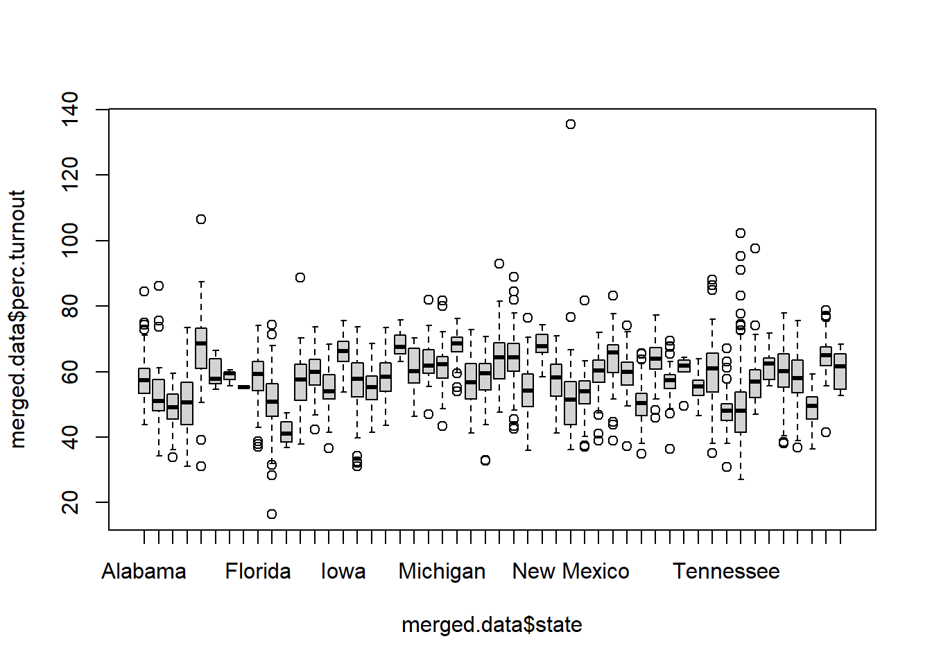
Hm, we’re still getting some points above 100, why is that??
ACS numbers are estimates! Things can get weird for very small counties where it may look like more than 100% of people are voting.
Let’s recode all values above 100 to 100/l
merged.data$perc.turnout[merged.data$perc.turnout>100] <- 100
boxplot(merged.data$perc.turnout ~ merged.data$state, outline=F)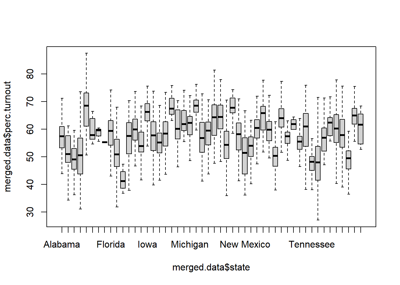
Is this a good or correct decision? To recode places about to 100 to 100? I think it’s a good one, but the rule is less “always do it this way” and more “be transparent”. This is a decision I would note in my script, and one that I would note in any report I was writing on this.
What if we wanted to do this for every year in the original elect dataset? That is, what if we wanted to merge in the county population figures for every observation in elect.all which is for all elections from 2000-2016.
Now there are 5 different Autagua Alabamas in the dataset. For each of these rows we want to merge in the vap number from our acs file. (Let’s ignore that this vap number would be changing over time for right now).
head(elect.all[order(elect.all$FIPS),])
#>       year   state  county FIPS totalvotes
#> 1     2000 Alabama Autauga 1001      17208
#> 3117  2004 Alabama Autauga 1001      20081
#> 6234  2008 Alabama Autauga 1001      23641
#> 9351  2012 Alabama Autauga 1001      23932
#> 12468 2016 Alabama Autauga 1001      24973
#> 2     2000 Alabama Baldwin 1003      56480
This is actually really easy, because R will do all of the work for us with the same command. It will know that every time there is FIPS 1001 in the elect dataset it should put in the appropriate number from the acs dataset.
full.merge <- merge(elect.all, acs, by.x="FIPS",by.y="Geo_FIPS",all.x=T)
head(full.merge[order(full.merge$FIPS),])
#>   FIPS year   state  county totalvotes    vap
#> 1 1001 2000 Alabama Autauga      17208  41831
#> 2 1001 2012 Alabama Autauga      23932  41831
#> 3 1001 2016 Alabama Autauga      24973  41831
#> 4 1001 2004 Alabama Autauga      20081  41831
#> 5 1001 2008 Alabama Autauga      23641  41831
#> 6 1003 2008 Alabama Baldwin      81413 162430
That looks right!
We can think about the limits to this process though: we can have one dataset that has multiple rows for a merging variable, but the other dataset must have one and only one row for the merging variable. So here, the elect data has many rows for each FIPS code and the acs data has one row for each FIPS code. We couldn’t complete this merge if the acs data had multiple rows for each FIPS code.
What if we had ACS Data like this, where we have a new vap number for each election year:
acs.series <- rio::import("https://github.com/marctrussler/IDS-Data/raw/main/ACSSeries.Rds")
head(acs.series)
#>   Geo_FIPS    vap year
#> 1     1001  39249 2000
#> 2     1003 162016 2000
#> 3     1005  18659 2000
#> 4     1007  21349 2000
#> 5     1009  43670 2000
#> 6     1011   6169 2000
How can we perform this merge? Now we have multiple FIPS codes for each year….
Thinking back to units of analysis, we are interested in what variable (or sets of variables) uniquely identifies rows. In both cases now the combination of FIPS and year uniquely identifies cases. So now we want to merge on both variables: matching FIPS 1001 in year 2000 to FIPS 1001 in year 2000 etc.
There are two ways to do this.
First we can create a new variable that simple combines these two variables into a new variable:
acs.series$county.year <- paste(acs.series$Geo_FIPS,acs.series$year,sep="")
head(acs.series)
#>   Geo_FIPS    vap year county.year
#> 1     1001  39249 2000    10012000
#> 2     1003 162016 2000    10032000
#> 3     1005  18659 2000    10052000
#> 4     1007  21349 2000    10072000
#> 5     1009  43670 2000    10092000
#> 6     1011   6169 2000    10112000
elect.all$county.year <- paste(elect.all$FIPS,elect.all$year,sep="")
head(elect.all)
#>   year   state  county FIPS totalvotes county.year
#> 1 2000 Alabama Autauga 1001      17208    10012000
#> 2 2000 Alabama Baldwin 1003      56480    10032000
#> 3 2000 Alabama Barbour 1005      10395    10052000
#> 4 2000 Alabama    Bibb 1007       7101    10072000
#> 5 2000 Alabama  Blount 1009      17973    10092000
#> 6 2000 Alabama Bullock 1011       4904    10112000
#If the variable is called the same thing in both datasets you don't have to do by.x and by.y:
merge.series <- merge(elect.all,acs.series, by="county.year", all.x=T)
head(merge.series)
#>   county.year year.x    state     county  FIPS totalvotes
#> 1   100012000   2000 Delaware       Kent 10001      48247
#> 2   100012004   2004 Delaware       Kent 10001      55977
#> 3   100012008   2008 Delaware       Kent 10001      66925
#> 4   100012012   2012 Delaware       Kent 10001      68696
#> 5   100012016   2016 Delaware       Kent 10001      74598
#> 6   100032000   2000 Delaware New Castle 10003     212995
#>   Geo_FIPS    vap year.y
#> 1    10001 133347   2000
#> 2    10001 134028   2004
#> 3    10001 134468   2008
#> 4    10001 134360   2012
#> 5    10001 134211   2016
#> 6    10003 435787   2000
This works ok, but note that we now have copies of FIPS and year now. Indeed, because there was the variable year in both datasets R has changed the names to year.x and year.y. Now we could fix this with some cleanup (or deleting out the FIPS and year variables from one of the datasets before merging).
The other way of doing this is to simply explicitly merge on both variables:
#Going to delete the merging variable we made first:
elect.all$county.year <- NULL
acs.series$county.year <- NULL

merge.series2 <- merge(elect.all, acs.series, by.x=c("FIPS","year"), by.y=c("Geo_FIPS","year"))
head(merge.series2)
#>    FIPS year    state     county totalvotes    vap
#> 1 10001 2000 Delaware       Kent      48247 133347
#> 2 10001 2004 Delaware       Kent      55977 134028
#> 3 10001 2008 Delaware       Kent      66925 134468
#> 4 10001 2012 Delaware       Kent      68696 134360
#> 5 10001 2016 Delaware       Kent      74598 134211
#> 6 10003 2000 Delaware New Castle     212995 435787