14 Causal Inference
We have already talked about “omitted variable bias” in this textbook in the context of regression. In that case we were thinking about adding variables to our regression that are a common cause of both the dependent and independent variables. We were doing this to isolate the “real” effect of our independent variable of interest on the dependent variable.
But dealing with “omitted variables” is just one version of a much larger topic: Causal Inference. This is the branch of statistics that thinks a lot about how we can isolate the true effects of different variables. It is actually one of the newest branches of statistics, largely founded in the 1970s and coming to prominence in the last 20-30 years. In this section I am going to give you a small taste of the framework this branch of statistics uses to think about data.
One note before we dive in: this type of thinking is completely parallel to the sort of thinking we covered in What is Data? and Hypothesis Tests. In those chapters we discussed how we can measure the uncertainty about whether estimates in our sample help us learn about the population. Causal Inference is interested in: are the estimates we are making (whatever the sample size!) the right estimates to be making? Both parts are important, but don’t really overlap.
14.1 When does correlation equal causation?
I have mentioned before that I’m not a huge fan of “correlation doesn’t equal causation.” By this, people usually mean that just because two things happen in concert doesn’t mean that one causes the other. It’s a technically correct statement, but is often wielded to dismiss any study that someone doesn’t like.
The truth of the matter is that no research design can actually prove causality. Instead of thinking of causality like something that either exists (x definitely causes y) or doesn’t (x and y are correlated but we don’t know if the relationship is causal) we can think about it like a continuum. We can have research designs that approximate causality to more or less degree.
The goal of this textbook section is to break down what “to cause” really means, and how we can apply that knowledge in regression and other research designs.
14.2 What does it mean for one thing to cause another thing?
The best way to think about what “cause” really means is to think about a light switch. Imagine getting up from your desk right now and walking over to the light-switch on the wall and flipping it. If you do so, almost certainly the light is going to go off. Now: does the light switch cause the light to turn off? Clearly, you are going to say that it does. But do we know that for certain? What if the power for the whole building went off right when you flipped the switch? What if the lights in the building are on a timer that happened to trigger right when you flipped the switch? While both of these things are implausible, they are possible.
So what information would we need in order to know with 100% certainty that the light switch turns the light on and off?
To know for certain what we would need to do is to both hit the light switch and not hit the light switch at exactly the same time. If we were able to do that, we would be able to see that hitting the light switch turns off the lights, and in the absence of us hitting the light switch the light, in fact, stays on.
We can extend this same logic to something like a drug trial. Let’s say that we have an individual who is experiencing some sort of ailment that we want to treat with our new drug. We give them the drug, monitor their progress, and after a few days they get better! So does the drug work?
Well… we don’t actually know! Similar to the light-switch: we don’t know what would have happened if we had not given them the drug! Maybe the drug worked and that’s why they were going to get better, but maybe they were going to get better anyways and the drug did nothing…
Again: the only way to really know if the drug works is to both give an individual the drug and to not give the same individual the drug at exactly the same time.
As an aside, this is actually what the “placebo” effect is. People believe that the placebo effect is that when you give someone a sugar pill their brain “makes” that drug work. This is true to some extent but not what the majority of the placebo effect is. What is actually happening is that people who are likely to enter into a drug trial are particularly sick. Because they are particularly sick when they enter the trial they will, without any intervention, get better on average. The placebo effect is just tracking these individuals’ regression to their usual level of sickness.
To formalize this we can think about two measures for a particular individual:
\(Y_{treat}\) is the outcome for an individual (something like their health in a drug trial) if they are treated.
\(Y_{control}\) is the outcome for an individual (somethign like their health in a drug trial) if they are not treated.
As such, the “treatment effect” is the difference between these two values:
\[ \delta = Y_{treat} - Y_{control} \]
The problem/abusrdity with this setup should be abundantly clear to you by now: absent a time machine we can never measure both \(Y_{treat}\) and \(Y_{control}\) for the same individual.
This is what is known as the Fundamental Problem of Causal Inference. The literal impossibility of this problem is why no research design ever captures the true causal effect.
14.3 What if we have lots of people?
For an individual person it is impossible to tell whether a drug works, or not. What if we have a lot of people? Is there something with aggregation that we can do to suss out causality in a situation like a drug trial?
Let’s pretend it is 2020 and we are in charge of determining whether the COVID-19 vaccines are effective or not.
One way of answering this question is to go out and survey people. We do everything right and get a random sample of a few thousand Americans and ask whether they have received the vaccine (are treated) or not (control). We also ask how many times they have gotten COVID, and calculate the average number of COVID cases among those who took the vaccine (\(\hat{Y}_T\)) and among those who did not take the vaccine (\(\hat{Y}_C\)).
We can then estimate the treatment effect as:
\[ \delta_n = \hat{Y}_T - \hat{Y}_C \]
This looks a lot like our equation above for the ideal treatment effect for an individual person. Above we couldn’t calculate that number because we couldn’t observe a person in both treated and untreated states, but now we have people in both states (those who took the vaccine and those who didn’t). Plus this sample was generated by randomly selecting people. So is this a good estimate of whether the vaccine is effective?
No it’s not!
At the individual level the Fundamental Problem of Causal Inference is that we cannot observe units in both their treated and untreated states. That’s a problem because we want to compare what happens when an individual is treated to what would have happened if they were untreated.
This aggregate version only works if the individual’s in the control group tell us what would have happened to the people in the treatment group if they had not taken the vaccine. Is that true? Are people who decided to not take the vaccine just like the people who did take the vaccine. Definitely not! These are two very different groups of people.
In particular, those who did not take the vaccine were also those who were more likely to get COVID in the absence of the vaccines (because of their behavior). So in the above calculation when we find that the treatment group has less COVID cases then the control group, a good chunk of that effect would exist with or without vaccines.
We can generalize this problem as one where certain types of people “select” a treatment making the resulting comparison to a “control” group biased.
Does political party cause individuals to abide by COVID precautions?
Does being from a wealthier district cause legislators to vote for lower taxes?
Do policies like Larry Krasner’s lead to a rise in crime in the US cities?
Does Tom Brady’s TB122 workout program help teams win the Superbowl?
In trying to determine the effects of all of these things we can think of reasons why a non-random group would “select” treatment, such that we can’t just compare those those who are treated to those that are not and get a good estimate of a treatment effect.
14.4 So how do we do it?
This seems like a really hopeless situation! We don’t have a time machine, and in many situations the things we are interested in are things that a non-random group of people select into…
But this thinking has at least allowed us to see what we need to have in order to show causality. In order to have an estimate of the treatment effect that is accurate, we must have a control group whose outcomes are equal to what would have happened in the treatment group had they not been treated.
So how do we do that?
We might think we should do some sort of “matching” procedure. We list out the characteristics of people who were treated, and then go and find exact matches of people just like them but who were not treated. This actually does exist, but as you can imagine it is really expensive! Further, this has the downside where we can only match on things that we can actually measure.
The real solution is way easier: Randomization is the solution to the Fundamental Problem Of Causal Inference.
If people are randomly assigned to treatment and control groups then, by definition, the two groups will be equivalent on all possible characteristics, whether we measure them or not.
This logic breaks down for very small groups – with 10 people you could imagine randomly assigning a weird group of 5 to treatment – but once you get to a sufficiently large group (like… 30) random assignment necessarily leaves with you two groups that are statistically equivalent. If you then assign treatment to one of those two groups then the only reason they are different is due to the treatment you give them.
14.5 Causal Inference as a missing data problem
As an example, we can think about a job training program that is set up for adults to be trained in a new skill-set.
The people funding the program want to know whether or not the program is helping participants get better paying jobs a year after they complete the program.
Consider these data, where for 10 people we know whether they were treated with this job program:
df <- data.frame(treat = c(T, T, F, T, F, F, F, T, T, F), y.obs = c(84000, 70000, 44000, 56000, 59000, 53000, 61000, 61000, 64000, 54000))
kableExtra::kable(df)| treat | y.obs |
|---|---|
| TRUE | 84000 |
| TRUE | 70000 |
| FALSE | 44000 |
| TRUE | 56000 |
| FALSE | 59000 |
| FALSE | 53000 |
| FALSE | 61000 |
| TRUE | 61000 |
| TRUE | 64000 |
| FALSE | 54000 |
If we think about measuring the outcome among the treated group and among the non-treated group we can see that what we have is a missing data problem:
df$y.treat[df$treat]  <- df$y.obs[df$treat]
df$y.control[!df$treat]  <- df$y.obs[!df$treat]
df$treat.effect <- NA
kableExtra::kable(df)| treat | y.obs | y.treat | y.control | treat.effect |
|---|---|---|---|---|
| TRUE | 84000 | 84000 | NA | NA |
| TRUE | 70000 | 70000 | NA | NA |
| FALSE | 44000 | NA | 44000 | NA |
| TRUE | 56000 | 56000 | NA | NA |
| FALSE | 59000 | NA | 59000 | NA |
| FALSE | 53000 | NA | 53000 | NA |
| FALSE | 61000 | NA | 61000 | NA |
| TRUE | 61000 | 61000 | NA | NA |
| TRUE | 64000 | 64000 | NA | NA |
| FALSE | 54000 | NA | 54000 | NA |
For those individuals who are treated we do not know what there value would be if they are in the control group, so that information is missing. The opposite is true for those who are not treated: we know what their value is for the control group but we do not know what their value would have been if they are in the treatment group.
Random assignment allows us to make the assumption that the average value among the control group is a good stand-in for the missing value for those in the treatment group and vice versa. The average value among the treated and control are:
So if we think about the first individual, our best guess for what would have happened to them if they were in the control group is that they would have made $54,200. For the third individual our best guess of what would have happened if they were in the treatment group is that they would have made $67,000. We can fill in all these values
df$y.treat[is.na(df$y.treat)] <- mean(df$y.treat,na.rm=T)
df$y.control[is.na(df$y.control)] <- mean(df$y.control,na.rm=T)
kableExtra::kable(df)| treat | y.obs | y.treat | y.control | treat.effect |
|---|---|---|---|---|
| TRUE | 84000 | 84000 | 54200 | NA |
| TRUE | 70000 | 70000 | 54200 | NA |
| FALSE | 44000 | 67000 | 44000 | NA |
| TRUE | 56000 | 56000 | 54200 | NA |
| FALSE | 59000 | 67000 | 59000 | NA |
| FALSE | 53000 | 67000 | 53000 | NA |
| FALSE | 61000 | 67000 | 61000 | NA |
| TRUE | 61000 | 61000 | 54200 | NA |
| TRUE | 64000 | 64000 | 54200 | NA |
| FALSE | 54000 | 67000 | 54000 | NA |
This allows us to determine, at the individual level, what the treatment effects are:
df$treat.effect <- df$y.treat - df$y.control
kableExtra::kable(df)| treat | y.obs | y.treat | y.control | treat.effect |
|---|---|---|---|---|
| TRUE | 84000 | 84000 | 54200 | 29800 |
| TRUE | 70000 | 70000 | 54200 | 15800 |
| FALSE | 44000 | 67000 | 44000 | 23000 |
| TRUE | 56000 | 56000 | 54200 | 1800 |
| FALSE | 59000 | 67000 | 59000 | 8000 |
| FALSE | 53000 | 67000 | 53000 | 14000 |
| FALSE | 61000 | 67000 | 61000 | 6000 |
| TRUE | 61000 | 61000 | 54200 | 6800 |
| TRUE | 64000 | 64000 | 54200 | 9800 |
| FALSE | 54000 | 67000 | 54000 | 13000 |
And the average of this column is our treatment effect:
mean(df$treat.effect)
#> [1] 12800
The purpose of this exercise was for you to conceptualize about how we use the treatment and control groups to stand in for the missing values for each other. In the “real” world we don’t have to go through all this work to get the treatment effect. If we have random assignment we just have to do:
t.test(df$y.obs ~ df$treat)
#>
#>  Welch Two Sample t-test
#>
#> data:  df$y.obs by df$treat
#> t = -2.2649, df = 6.6392, p-value = 0.05993
#> alternative hypothesis: true difference in means between group FALSE and group TRUE is not equal to 0
#> 95 percent confidence interval:
#>  -26312.4162    712.4162
#> sample estimates:
#> mean in group FALSE  mean in group TRUE
#>               54200               67000
We can alternative do:
lm(df$y.obs ~ df$treat)
#>
#> Call:
#> lm(formula = df$y.obs ~ df$treat)
#>
#> Coefficients:
#>  (Intercept)  df$treatTRUE
#>        54200         12800
14.6 Two types of randomness to remember
There are two types of randomness that you need to remember that solve very different problems. It’s a good idea to commit to memory what they are and why they are important.
- Random Assignment to Treatment is the solution to the Fundamental Problem of Causal Inference. This helps us get unbiased estimates of treatment effects by creating two groups that are identical except for one being exposed to treatment.
- Random sampling is the critical step for building a samping distribution and being able to perform a hypothesis test. We need to know that the sample we have in front of us is one of many random samples we could have that are pulled from the same distribution in order to calculate a standard error.
14.7 The real world
It’s fine to say that randomization is the solution to the Fundamental Problem of Causal Inference, but what about situations where we can’t randomly assign treatment? What are the effects of someone’s political party on their COVID behavior? Or electing a progressive DA on crime? Or having Gestational Diabetes on the health outcomes for a newborn? In none of these situations can we “randomly” assign treatment.
In these situations our goal is still to compare those who are treated and those who are not treated in a way that the only difference between the groups is exposure to treatment.
There are some fancy ways that we try to do this literally. One is regression discontinuity, where we look at situations like this:
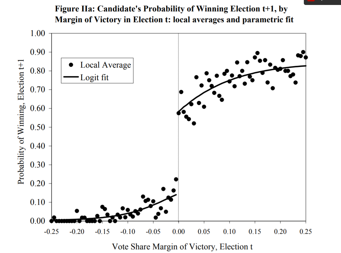
In this situation we want to know what the effect of winning an election in one time period is on winning subsequent elections. Like other situations here we can’t just compare people who have won an election to people who haven’t won an election to see how they do… people who win elections are winners! They are very likely to be different than the pool of “normal” candidates. They might be of higher quality, or be able to attract more money, or have policies that are closer to the median voter. All of these things violate the principle of having two groups that are equivalent except for treatment.
In the above graph we are looking at a group of people who ran in two consecutive elections. On the x-axis are the results of the “first” election these candidates ran in, and on the y-axis are the results of the “second” election these candidates ran in. Thinking about the the x-axis, people to the left of the dotted center line lost their first election and people to the right of that line won their first election.
The logic of regression discontinuity is that if we compare people who are just barely to the left and to the right of that center line we approach a situation where the two groups are comparable, except for the fact that one group won their election. Put another way: the people just to the left and right of the line in the graph are very similar, except one group got a lucky break and won their first election. The graph shows that these people do a good amount better in the second election!
But the usefulness of techniques like Regression Discontinuity are pretty limited.
Instead, a more nuanced way to think about causality is to think about it as a continuum where we rule out factors that cause both selection into treatment and the outcome. Instead of thinking about “x definitely causes y”, a more fruitful place to be is “we’re not definitely sure that x causes y, but we’ve rules out z as a potential alternative explanation”.